Beginner’s Guide to Google Sheets with Video and Screenshots

Google Sheets is an amazing application that allows you to create and manage spreadsheets. It has over the years become a very powerful tool however, it can be daunting to get started with. There are a ton of features and functions and it can be very easy to get overwhelmed.

Fear not though! This beginner’s guide to Google Sheets will teach you everything you need to know to get started using this powerful application.

Before we get started with the tutorial, if you are looking to learn more about apps like Notion, Todoist, Evernote, Google Sheets, or just how to be more productive (like Keep Productive’s awesome Notion course), you should really check out SkillShare. Skillshare is an online learning platform with courses on pretty much anything you want to learn. To learn more about Skillshare and its vast library of courses and get 30% off, click the link below:

SkillShare – Online Learning Platform

Looking to learn how to use conditional formatting in Google Sheets? You have to check out our Ultimate Guide to Conditional Formatting in Google Sheets.

Now, let’s get started with the tutorial 😀.

Accessing Google Sheets

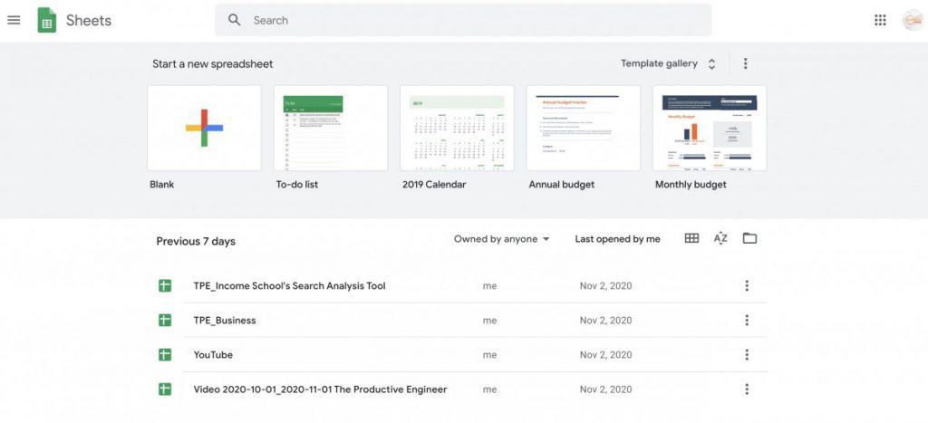
Google Sheets can be accessed by going to https://sheets.google.com. Once you have logged in using your Google/Gmail credentials, you should see a screen like the one above.

The main page of Google Sheets will display the last several spreadsheets you have used in the order from most recently edited to least recently edited.

Creating a New Spreadsheet in Google Sheets

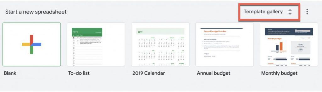
Google Sheets makes it really easy to jump right in and start using it. On the main page, you will be shown a “Start a new spreadsheet” section that allows you to either:

• Create a blank spreadsheet
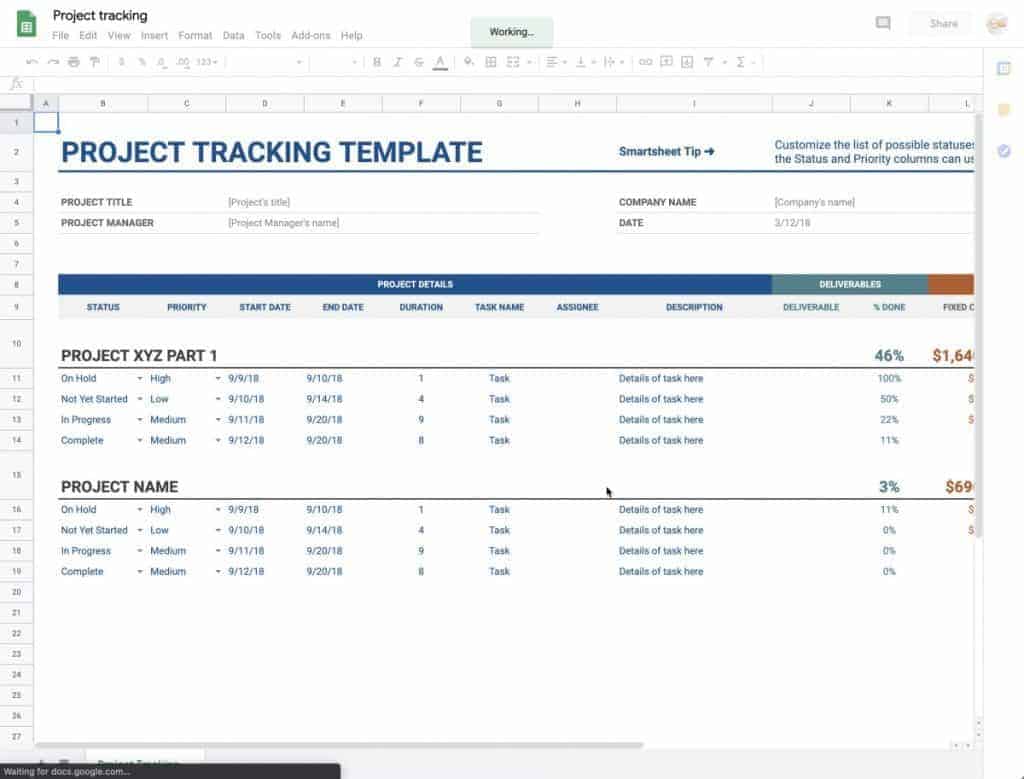
• Use a pre-made template

At least for me, I find myself just starting with a blank spreadsheet most of the time but it is nice to know that there are templates available if I need them.

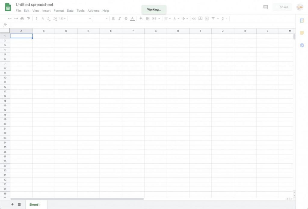
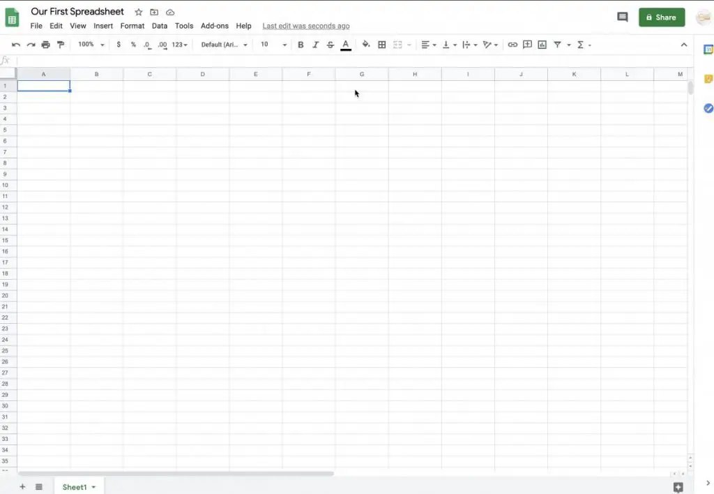
To create a new blank spreadsheet, simply click the “Blank” button. You should be presented with a blank spreadsheet as shown in the screenshot above.

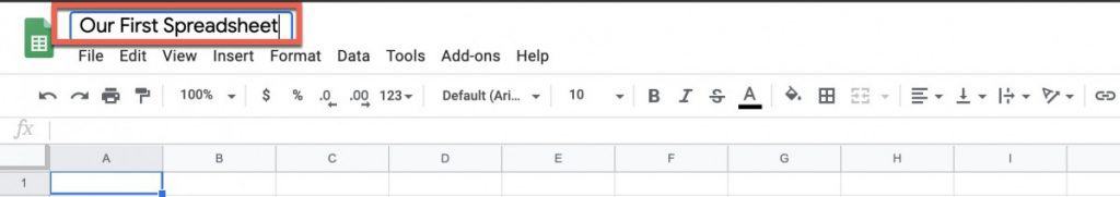
To add a title to your Google Sheets spreadsheet do the following:

1. Click on the text “Untitled Spreadsheet“
2. Select all the text by double-clicking your mouse button
3. Hit the Backspace key to delete the existing text
4. Type in your title
5. Hit the “Enter” key

Your spreadsheet should now show the new title you just gave it like the screenshot above for our example. This will be the file name for your spreadsheet. If you want to change it, you can by simply following the same instructions as before.

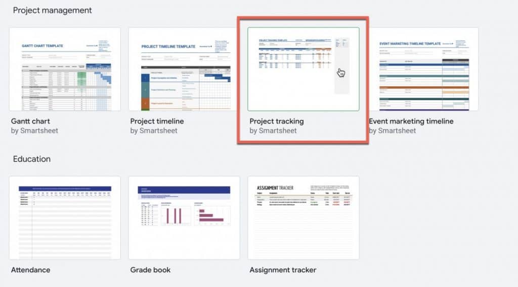
Using Pre-Built Templates in Google Sheets

As mentioned earlier, Google Sheets provides several templates to help get you started if you are looking for help getting started.

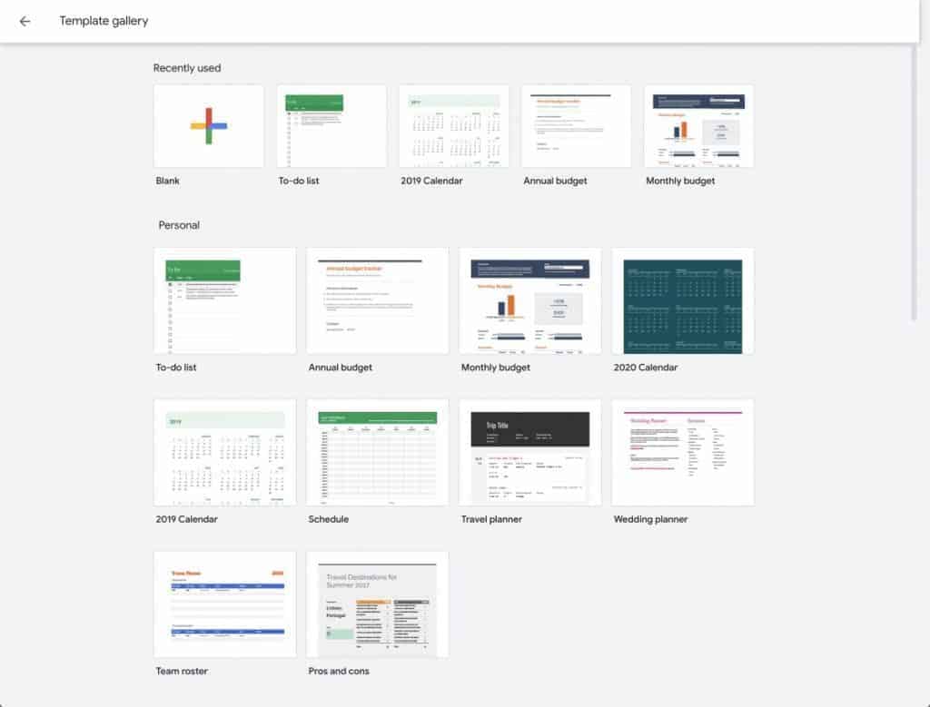
The four categories of templates in Google Sheets are:

• Personal
• Work
• Project Management
• Education

Adding a New Worksheet to a Google Sheet

There are three ways to add a new worksheet to a Google Sheets spreadsheet:

• Keyboard Shortcut Shift + F11
• Go to Main Menu and go to Insert -> New Sheet
• Click the “+” button in the bottom left corner of Google Sheets window

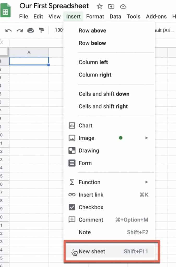
The quickest way to add a new sheet to your Google Sheets spreadsheet is to simply to press the Shift and F11 keys. Or you can use the main menu, navigate to the “Insert” menu and select “New sheet” as shown above.

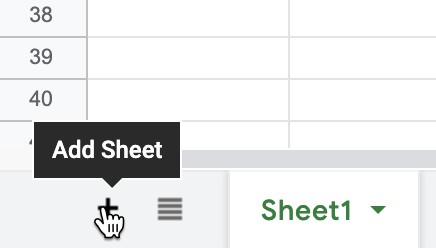
Alternately, you can simply press the “+” button in the bottom left hand corner of the Google Sheets window as shown in the screenshot above.

Editing Cells

Editing cells in Google Sheets is easy to do and follows the same structure as editing cells in Microsoft Excel or other spreadsheets.

Editing Text in Cells in Google Sheets

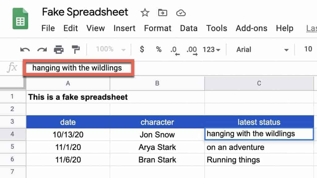
To edit or add some text to a cell in Google Sheets, simply click on the cell. You should see a blue box around the cell you have selected. As you can see in the screenshot above, there is a text box above the cells (it is highlighted in red in the screenshot). This is where you add or edit text to the cell.

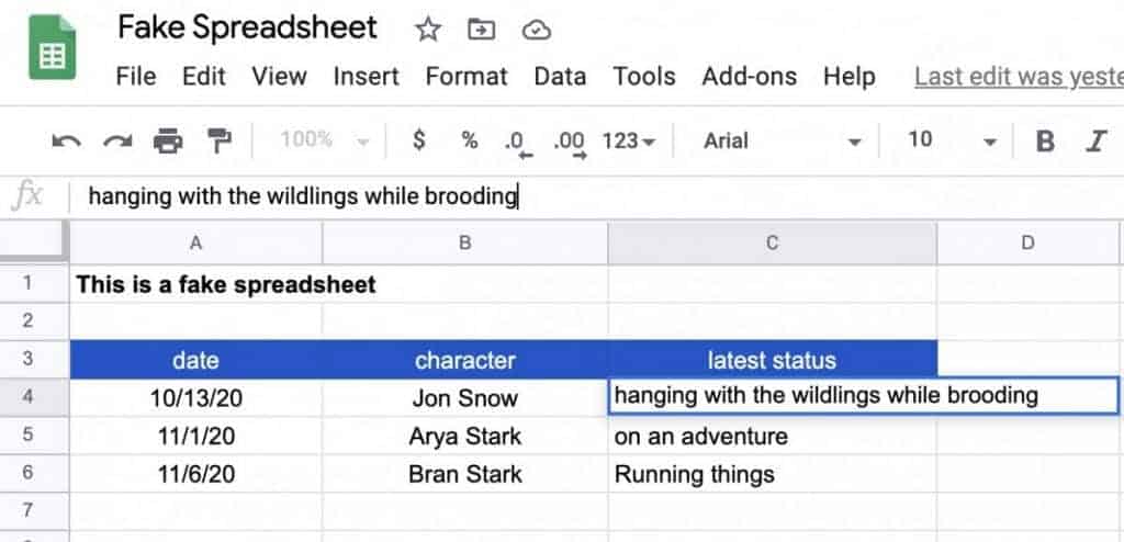
You can add text by simply clicking your cursor inside the text box and start typing. You should notice your text being added to the cell in real time as you type in the text box. To edit existing text, simply select it by clicking and dragging your mouse over the text you want to edit and start typing.

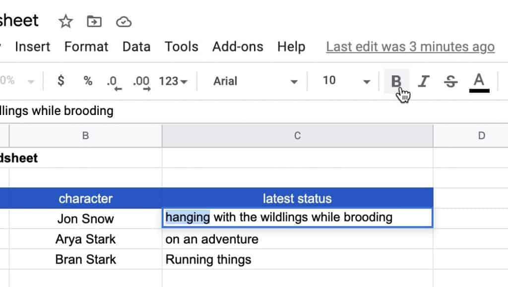
Text Formatting in Google Sheets

You may have noticed the text formatting bar (shown above). This is where you can add formatting to your text in Google Sheets. Enclosed below is each function in the text formatting toolbar in Google Sheets (from left to right in the toolbar above):

• Font Picker
• Font Size
• Bold
• Italic
• Strikethrough
• Text Color
• Cell Color
• Borders
• Merge Cells
• Horizontal Align
• Vertical Align
• Text Wrapping
• Text Rotation

You can use either the text formatting bar to format your text and cells or use the appropriate keyboard shortcut as shown in the table below:

Function	Mac Keyboard Shortcut	Windows Keyboard Shortcut
Bold	⌘ + b	Ctrl + b
Underline	⌘ + u	Ctrl + u
Italic	⌘ + i	Ctrl + i
Strikethrough	Option + Shift + 5	Alt + Shift + 5
Align Center	⌘ + Shift + e	Ctrl + Shift + e
Left Align	⌘ + Shift + l	Ctrl + Shift + l
Right Align	⌘ + Shift + r	Ctrl + Shift + r
Apply Border to top of cell	Option + Shift + 1	Alt + Shift + 1
Apply Border to right of cell	Option + Shift + 2	Alt + Shift + 2
Apply Border to bottom of cell	Option + Shift + 3	Alt + Shift + 3
Apply Border to left of cell	Option + Shift + 4	Alt + Shift + 4
Remove Borders	Option + Shift + 6	Alt + Shift + 6
Apply Outer Border	Option + Shift + 7 or ⌘ + Shift + 7	Alt + Shift + 7 or Ctrl + Shift + 7

Leveraging these text and cell formatting options is as easy as selecting text or cell and applying the function as shown below:

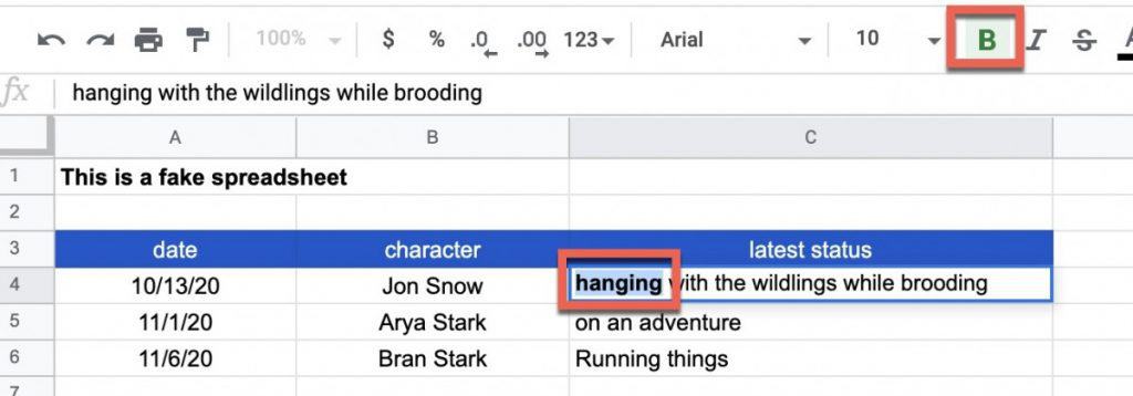
Try using some of the text formatting functions to see how they work. Try to use the keyboard shortcuts so that you learn them as they can save you some time.

Working with Numbers in a Cell in Google Sheets

The power of any spreadsheet application is how well you can work with numbers in it. Google Sheets is no exception as it offers a rich feature set for working with and manipulating numbers.

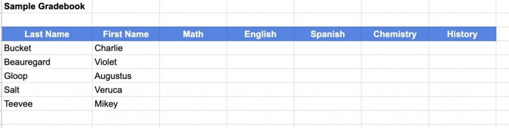
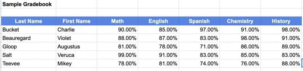
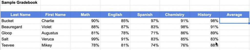
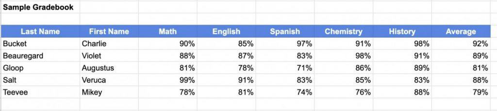
I have a simple grade book worksheet above. We are going to use this spreadsheet to show how we can work with numbers inside of Google Sheets.

Number Format Types in Google Sheets

The first thing we will cover is number formatting. Google Sheets supports a wide variety of number formatting options. Enclosed below is a list of some of the number formats Google Sheets supports:

• Number
• Percent
• Scientific
• Accounting
• Financial
• Currency
• Currency (rounded)
• Date
• Time
• Date time
• Duration

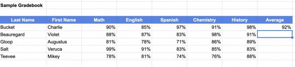
Let’s test number formatting by using our grade book spreadsheet. The spreadsheet contains grades in basic for each student for each class they have taken. Grades are typically given as a percentage so let’s format the grades as percentages.

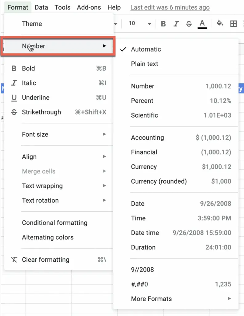
To format the grades as a percent in Google Sheets do the following:

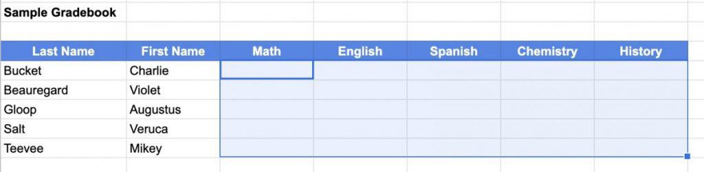
1. Select by clicking and dragging your mouse across the cells you want to show as a percent
   

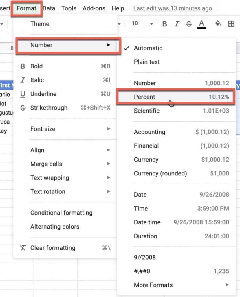
2. Go to Format -> Number and select Percent as shown in the screenshot above.

3. Enter the values you want for each student.

You should see them automatically formatted as percentages. The Percent option by default uses two decimal points of precision. If you don’t want decimals in your grades do the following:

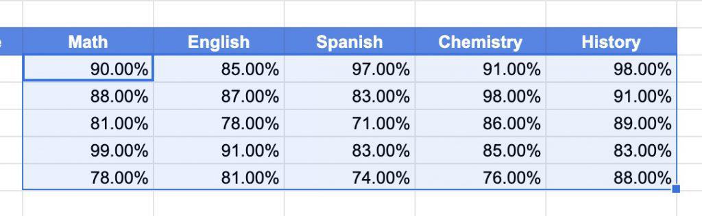
1. Select your values by clicking and dragging your mouse over the values you want to remove the decimals for

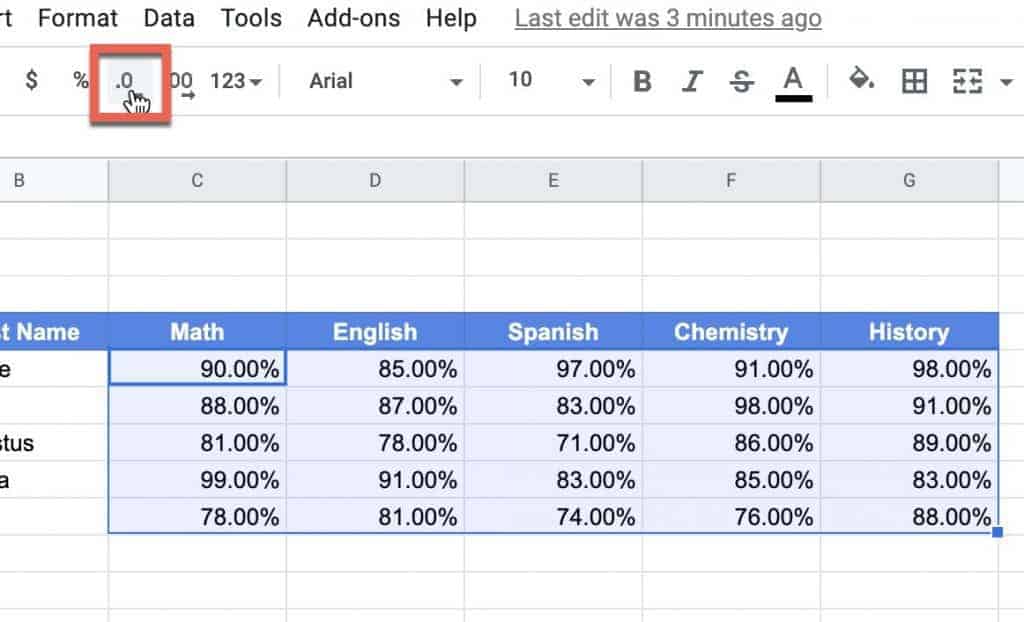
2. Click on the Decrease decimal button as shown above. In the case of our example, I would click the button twice as we have two decimal points of precision we need to remove

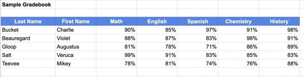
Our grade book now shows the grades as percentages with no decimal points. Next we will cover working with dates in Google Sheets.

Dates in Google Sheets

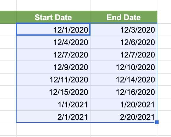
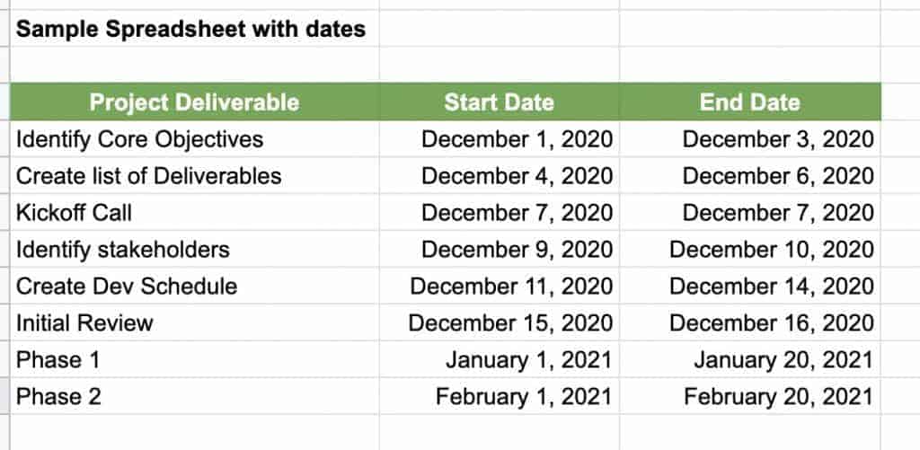
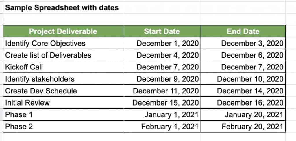
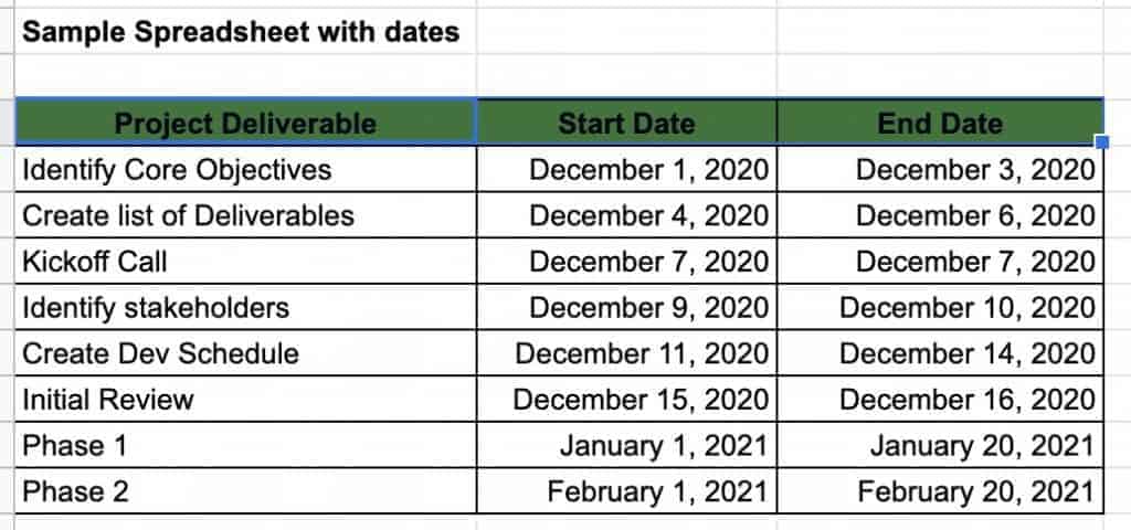
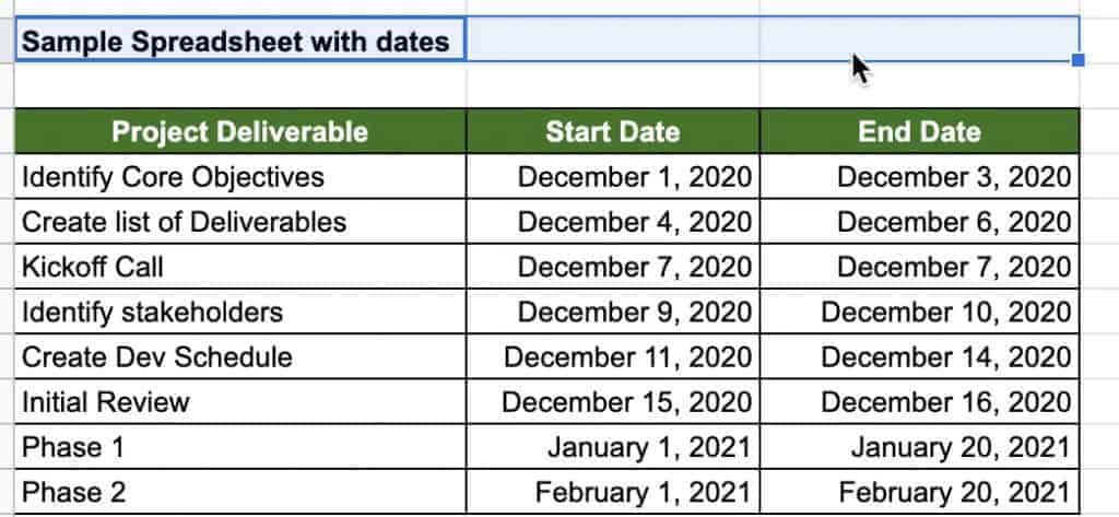
If you are doing any kind of project or task management in Google Sheets then you will need to know how to work with dates. Google Sheets makes it straight-forward to work with dates.

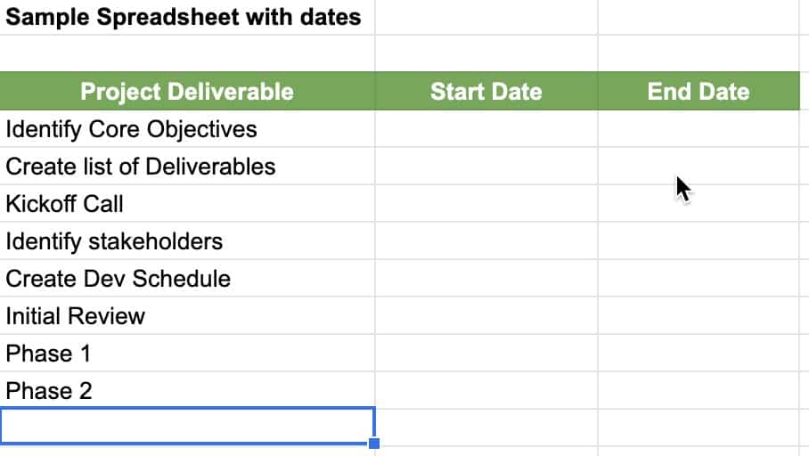
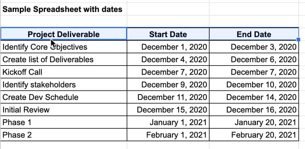
As you can see from above, I have created a quick project spreadsheet with two date columns:

• Start Date
• End Date

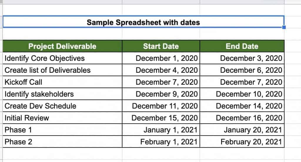
The first thing we want to do is to format the cells in those two date columns to be date fields. Google Sheets supports several options for how the date will appear.

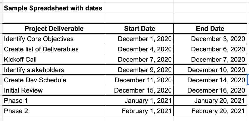
Let’s first start with the default date format.

Select the cells you want to format as dates by clicking and dragging your mouse across the cells.

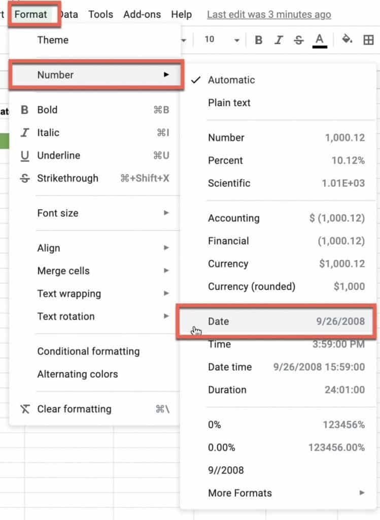
Go to Format -> Number and select the Date option from the menu.

But what if you want to change the date format to display the date in a different way? As I mentioned earlier, Google Sheets supports displaying the date in a number of different ways. To change the way the date is displayed in Google Sheets, do the following:

1. Select the dates you want to modify

2. Go to Format -> Number -> More Formats and select More date and time formats from the menu

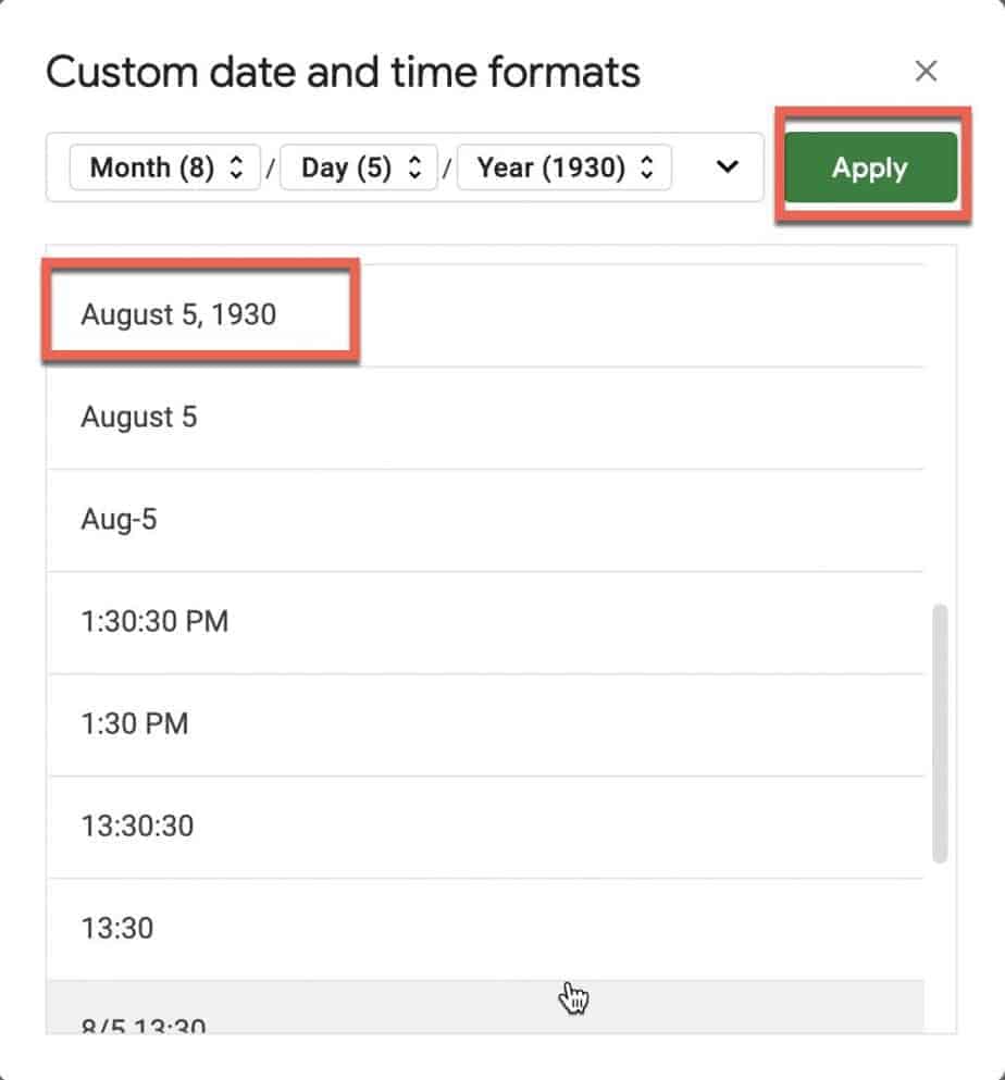
3. The Custom date and time formats dialog box will appear. Scroll down and select the format you want and click the Apply button.

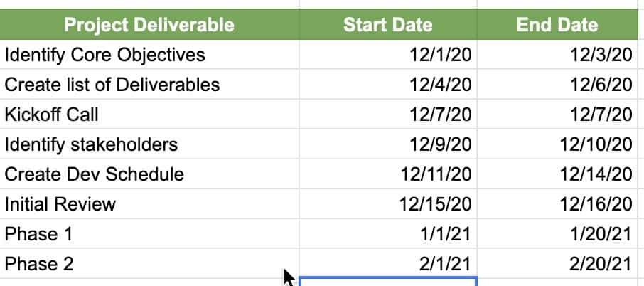
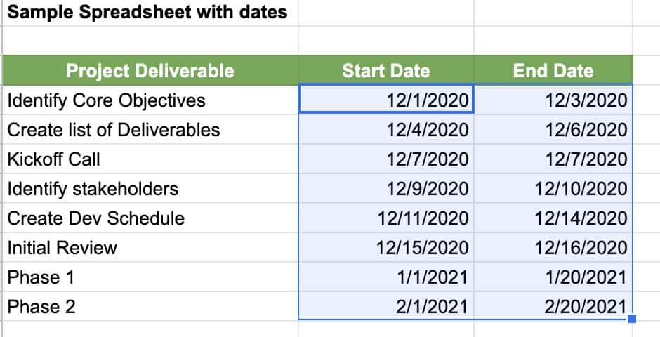
Your date fields will now be in the format you selected.

Adding Borders to Cells in Google Sheets

Google Sheets makes it easy to add borders to cells in your spreadsheet. To add borders to cells in Google Sheets, do the following:

1. Select the cells you want to apply a border(s) to

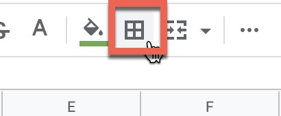
2. Click on the Border button in the toolbar as shown in the screenshot above

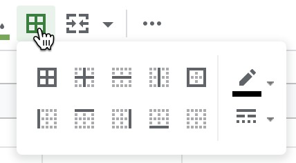
3. Select the border option you want from the pop-up dialog box. You can also specify the color and style/thickness of the borders using the color and style icons on the right side of the dialog box

Your selected cells should now have the border you chose.

Next, let’s learn how to add some color shading to cells in Google Sheets.

Adding Shading to Cells in Google Sheets

As you can see from the image above, a table without any background colors can look really boring. Adding a background color to cells in Google Sheets help the important content stand out. Whether it’s column headers or simply highlighting important cells, knowing how to shade cells in Google Sheets is an important skill.

To shade a cell in Google Sheets, do the following:

1. Select the cell(s) you want to shade

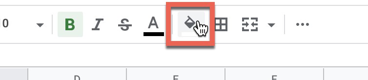
2. Click on the paint can button to bring up the color background picker

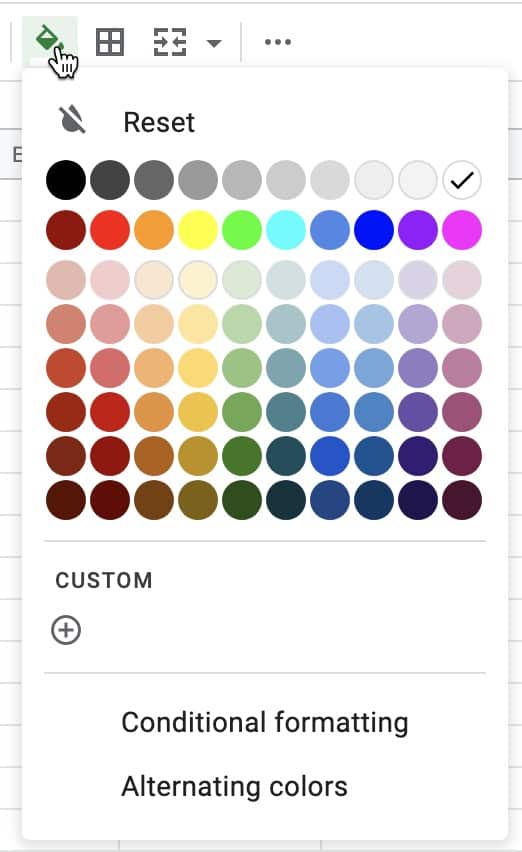
3. Choose the color by clicking on the color swatch you want

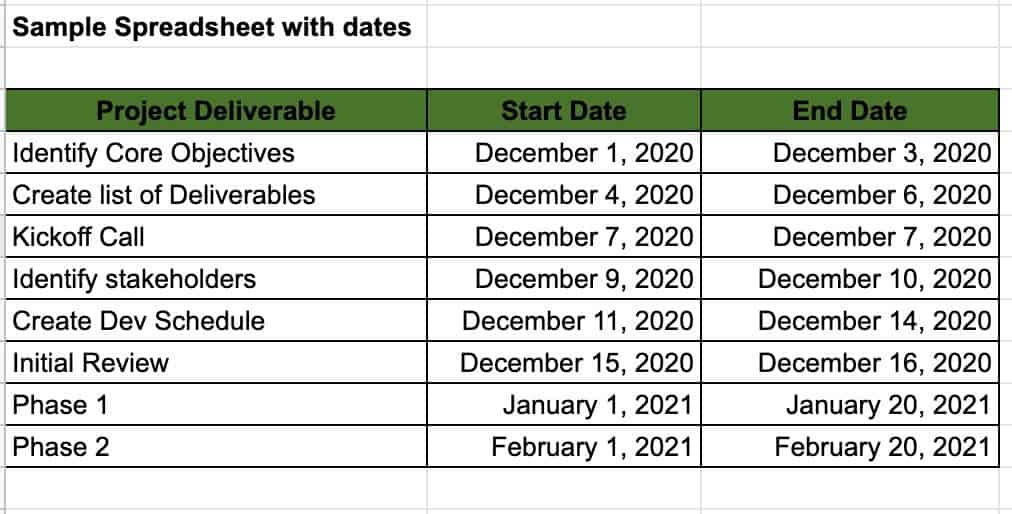
Your cells should now have a background color. But, do you notice that the black text is hard to read against the dark green background? Well, I do so let’s change the text color to white to make it more readable.

To change the text color in Google Sheets, do the following:

1. Select the cell(s) containing the text you want

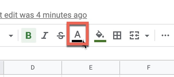
2. Click on the Text Color button to bring up the text color picker

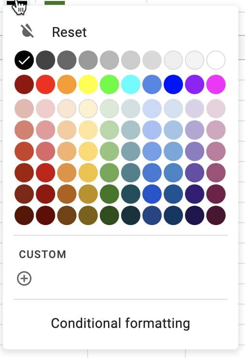
3. Pick the color you want your text to be by clicking on the color swatch of the color you want

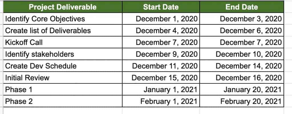
Your text will now be the color you selected. In our example, I changed the text color from black to white by selecting the white color swatch in the text color picker.

Next, let’s learn how to merge cells in Google Sheets.

Merging Cells in Google Sheets

Sometimes you need or want to format your cells in a way that requires you to merge two or more cells together. To merge two or more cells together in Google Sheets, do the following:

1. Select the cells you want to merge together

2. Go to Format -> Merge Cells and select either Merge all or Merge Horizontally depending on what you require

Your cells should now be merged into a single cell. As you can see from the image above, I am now able to center my text across the length of the table now due to merging the cells together.

We will now cover how to use images in Google Sheets.

Using Images in Google Sheets

Google Sheets provides two ways an image can be inserted into a spreadsheet:

• Image in cell
• Image over cell

We will cover both in the next two sections.

Images in cell

Using the images in cell option places the image inside of a cell. To place an image inside a cell in Google Sheets, do the following:

1. Select the cell that you want to place an image inside

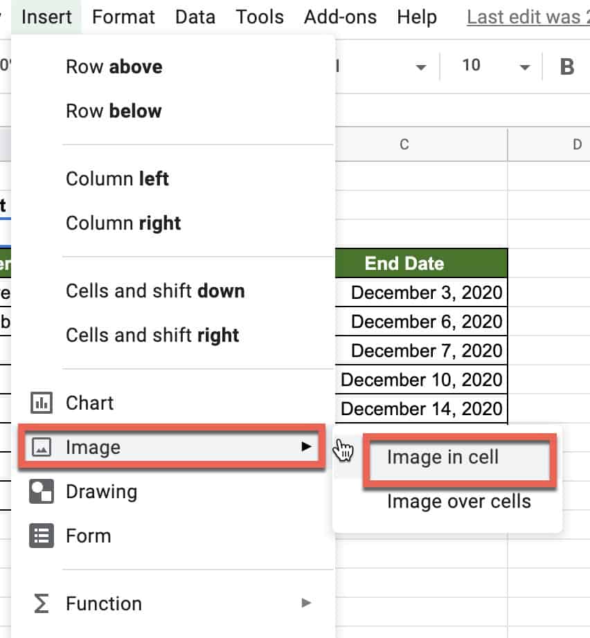
2. Go to Insert -> Image and select Image in cell from the menu

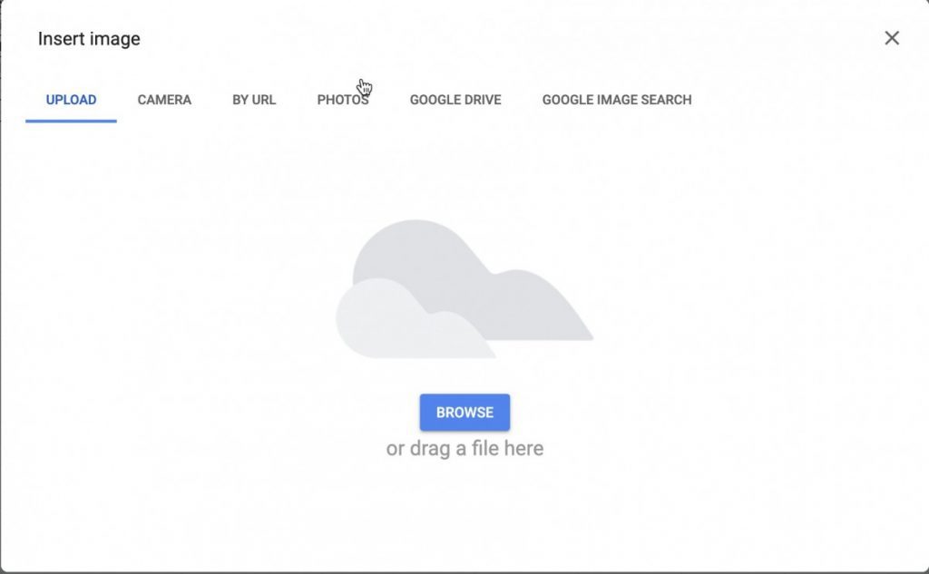
3. The Insert image dialog box will appear. Select the appropriate option for you. In our example we will choose Upload and clicking the Browse button.

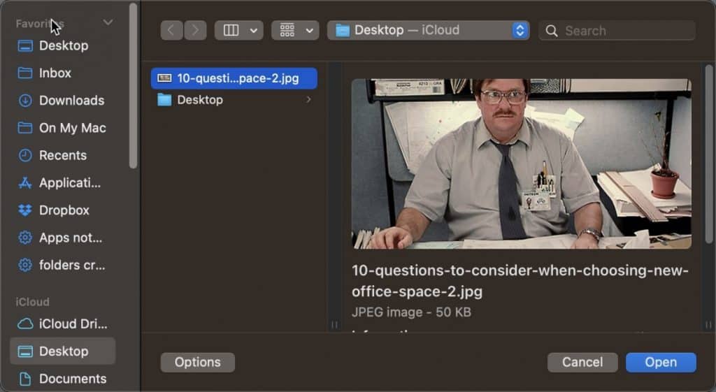
4. Select your image file and click “Open“

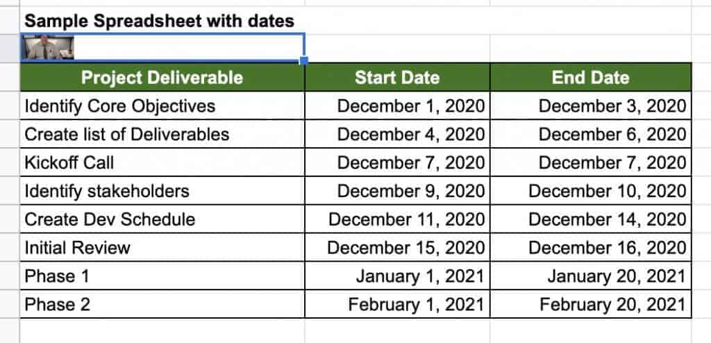
Your image will appear inside your cell.

The image will size itself to fit within the cell so to make the image bigger just resize the cell.

Images over cell

The Images over cell option will place the image over the top of the cell and will retain the size of the original image. Using this option will require you to create an adequate space prior to placing the image to ensure that the image doesn’t cover any content.

To add an image over cell in Google Sheets, do the following:

1. Pick out the area where you want to image to go. Resize the cell area to ensure it is big enough to hold the image

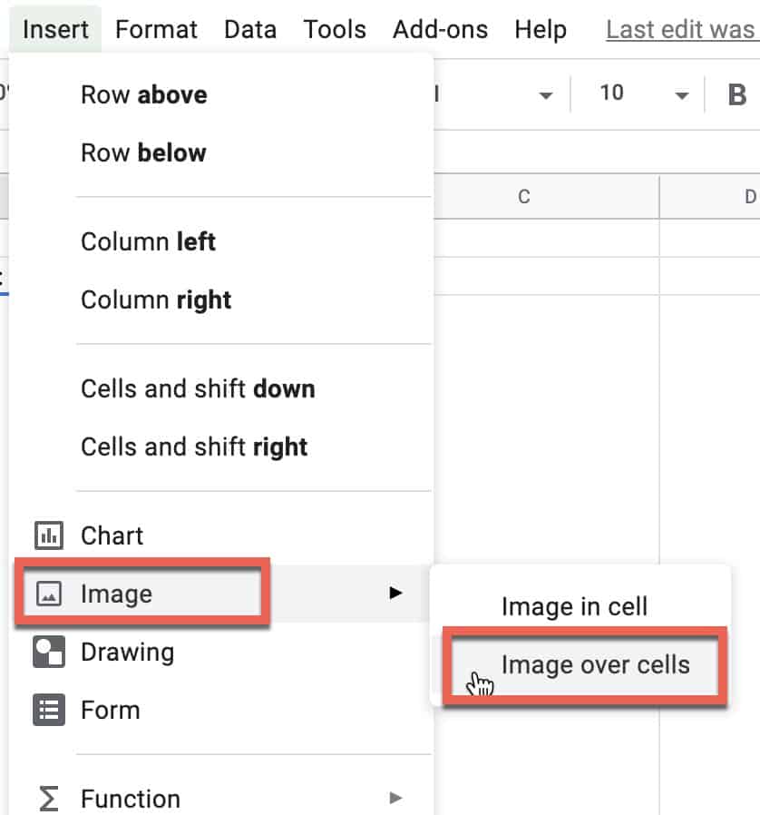
2. Go to Insert -> Image and select Image over cells from the menu

3. Select the appropriate option to get your image

4. Select your image and click “Open”

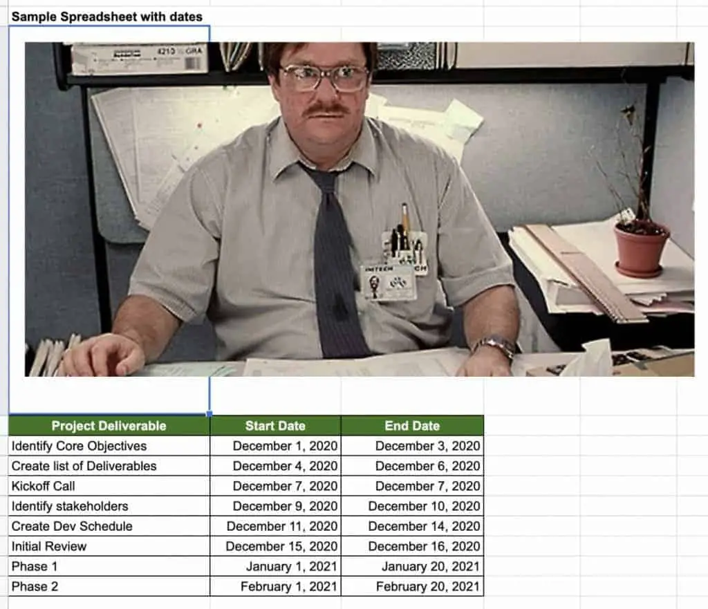
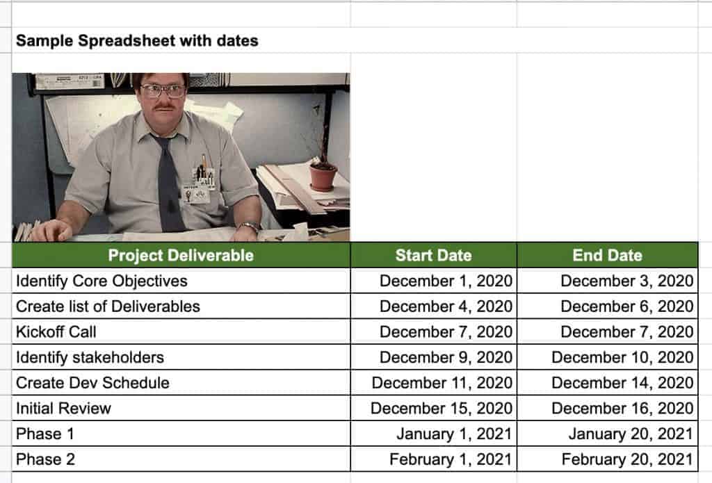
Your image will now be placed in the spreadsheet. Notice that the image is not constrained to a single cell but rather extends across cells.

Using Formulas in Google Sheets

If you are looking to do any sort of calculations in Google Sheets, you will need to familiarize yourself with formulas. Formulas allow you to perform calculations in Google Sheets. Google Sheets has a rich library of formulas to choose from but we will focus on a couple of key ones you will likely use over and over again.

How to Sum a Column or Row in Google Sheets

One of the most common tasks you will likely do in Google Sheets is to sum a bunch of values in a row or column. Google Sheets makes this very easy to do using the SUM() function.

To sum a row or column of values in Google Sheets, do the following:

1. Click on the cell where you want the sum to be

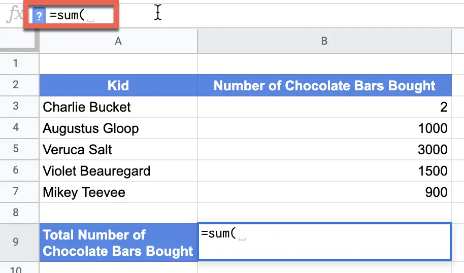
2. In the text box, type =SUM( as shown in the screenshot above

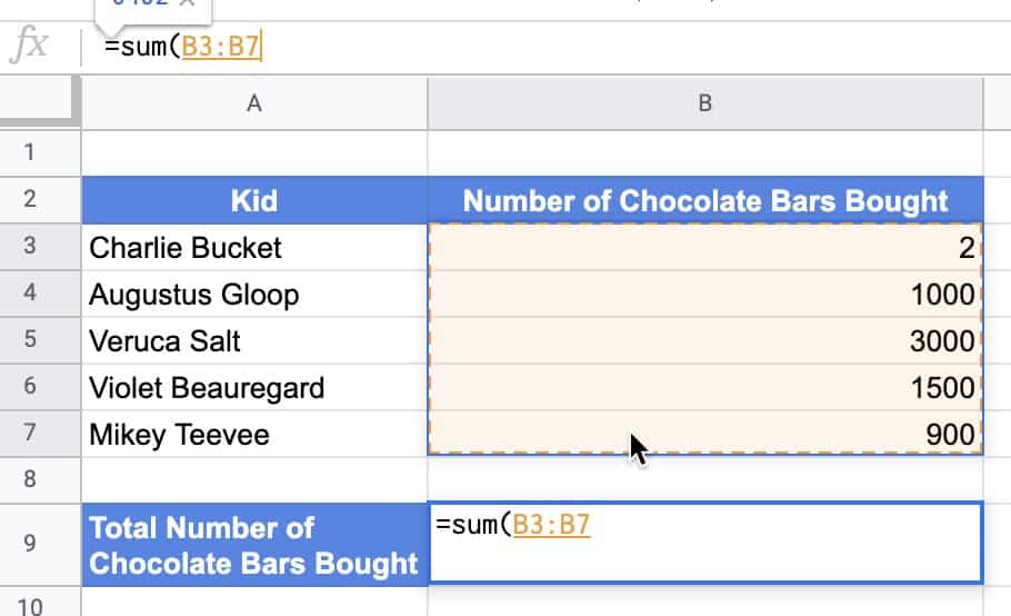
3. Click and drag your mouse across the cells you want to sum up.

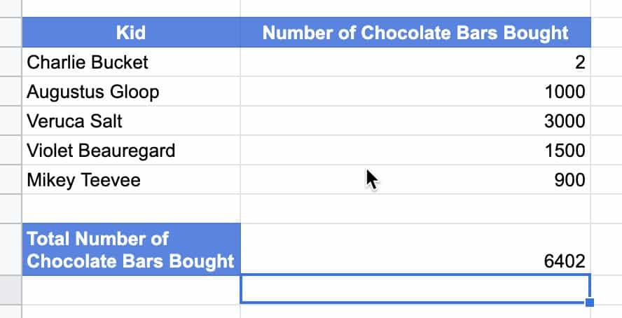
4. Hit the Enter key and you should now see the sum of the values you selected

This technique works for both summing rows as well as columns.

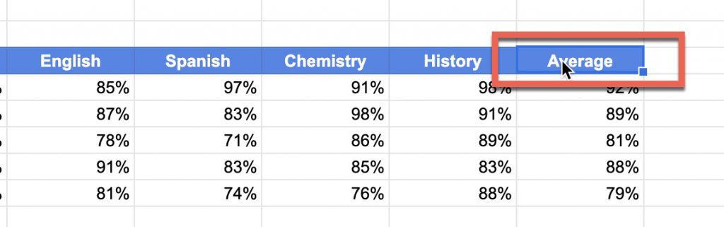
How to Average a Row or Column in Google Sheets

Another task you likely will find yourself doing in Google Sheets is calculating the average of a row or column of values. Again, Google Sheets makes it very easy to calculate the average of any number of values by using the AVERAGE() function.

To calculate the average of values in Google Sheets, do the following:

1. Select the cell where you want the average value to be

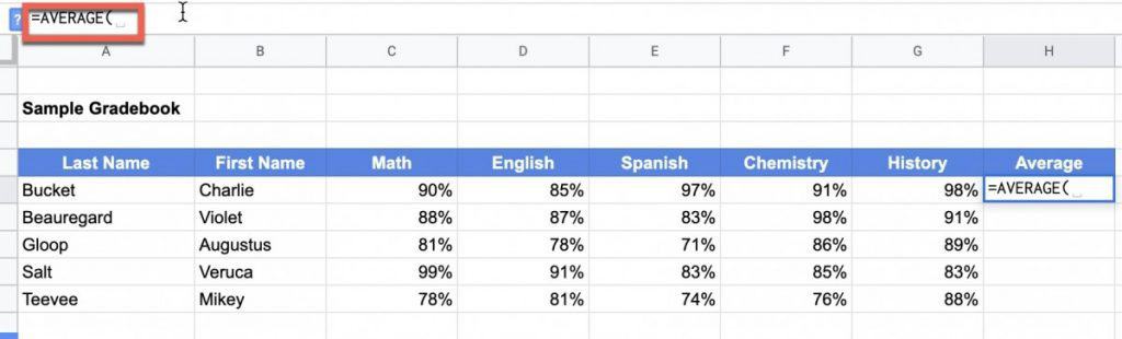
2. In the text box, type =AVERAGE( as shown above

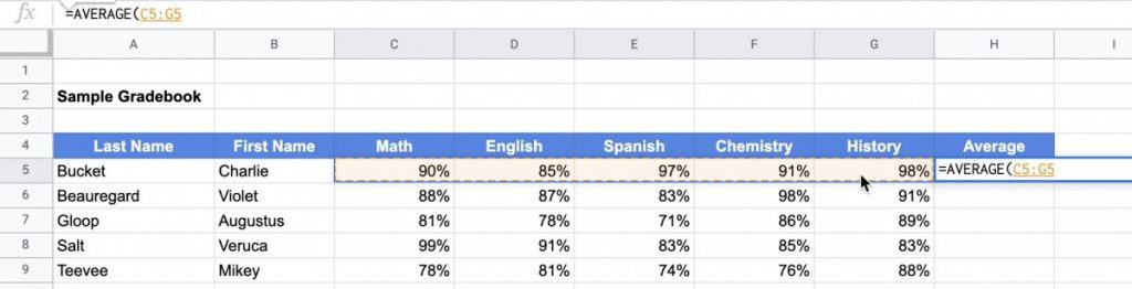
3. Select the cells you want to average by clicking and dragging your mouse across those cells as shown in the screenshot above.

4. Your average should appear in the cell.

Ninja trick, you can quickly apply the same formula (in our case AVERAGE) to the remaining rows.

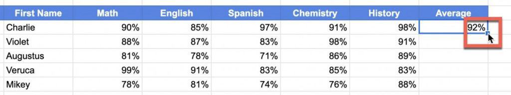
Select the cell that contains your formula. You should see a blue “dot” in the lower right hand corner of the cell.

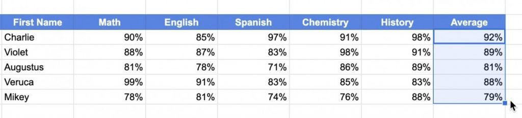
Click and drag that dot across all the cells where you want to apply the same formula. Google Sheets has the intelligence to apply the formula to the values in the appropriate cells.

Release the mouse button and your formula should now have been applied to all the other values you wanted. Pretty neat, huh?

Filters in Google Sheets

Filters allow you to see only the content you want to see in a spreadsheet. Filters are a very powerful tool once you learn how to work as they help you narrow down what you see to only the content that is relevant to you in that moment.

To create a filter in Google Sheets, do the following:

1. Click on the column heading you want to filter

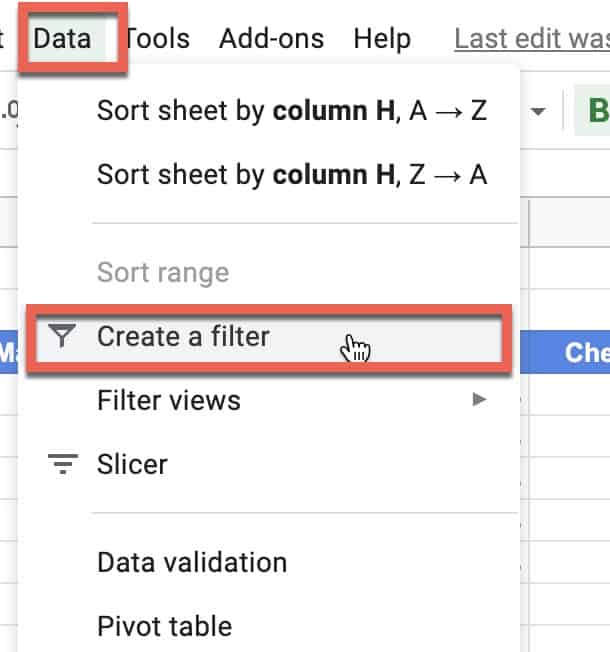
2. Go to Data and select Create a filter from the menu

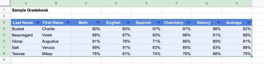
3. You should now see filter icons to the right of each column header

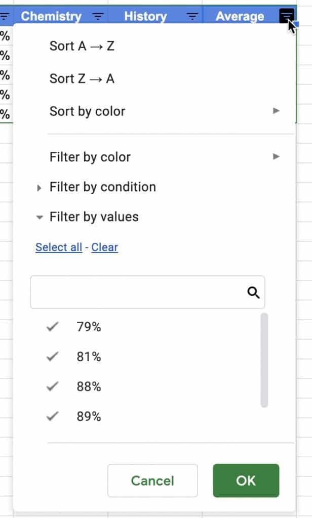
4. Click on the filter icon for the column you want to filter on. You will see a menu appear like the one above

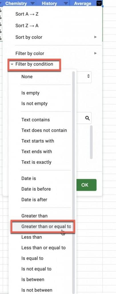
5. Select the criteria you want to filter on. In our example, I want to see all the students whose grade average is greater than or equal to 90 (in other words, an A student) so I chose Greater than or equal to under the Filter by condition option as shown above.

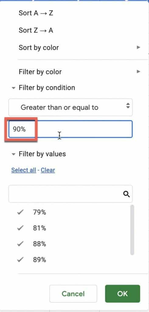
6. Fill in the value you want (in our case, 90%) and click OK.

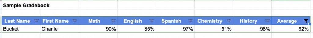
7. As you can see, the filter now only shows the student entry whose has an average of 90% or greater.

This is just one example of how you can use filters to sort and view data in Google Sheets. I recommend that you experiment on your own to see all the things you can do with filters.

Check out our Resources page

Check out our resources page for the products and services we use everyday to get things done or make our lives a little easier at the link below:

Link to resources page

Check Out Our YouTube Channel!

We have a YouTube channel now and we are working hard to fill it with tips, tricks, how-tos, and tutorials. Click the link below to check it out!

link to our YouTube page

Subscribe to Our Newsletter

If you like this article, subscribe to our newsletter. It contains tips and tricks to help you get things done.

Looking to Get Started Blogging or on YouTube?

Getting started can seem daunting and scary (I know it was for me) but it doesn’t have to be. I was very lucky to find a program that that has helped me grow my blog to over 60,000 page views and a monetized YouTube channel that is growing at over 100% month-over-month.

Income School is the program that I have used. I have been a member for over a year now and just renewed my membership. I cannot recommend Income School enough! For more information on Income School, click the link below:

Income School – Teaching You How to Create Passive Income from Blogs and YouTube