How to Make a Pie Chart in Google Sheets

Pie charts are a popular visual aid for presenting parts of a whole. They help to present data in a clear and easily understandable way. Creating pie charts in Google Sheets is straightforward and can really help make your data more digestible. This tutorial will teach you how to create pie charts in Google Sheets.

To create a pie chart in Google Sheets, do the following:

1. Select the data to be used for the pie chart
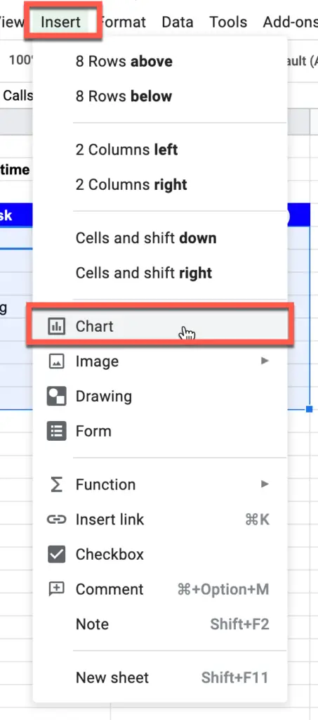
2. Go to the menu item Insert, and from the drop-down menu, select Chart.
3. Enter the chart data, and your pie chart will be generated automatically.

Before we get started with the article, if you are looking to learn more about apps like Notion, Todoist, Evernote, Google Docs, or just how to be more productive (like Keep Productive’s awesome Notion course), you should really check out SkillShare. Skillshare is an online learning platform with courses on pretty much anything you want to learn. To learn more about Skillshare and its vast library of courses and get 30% off, click the link below:

SkillShare – Online Learning Platform

Looking to get more proficient in Google Sheets? Check out our Beginner’s Guide to Google Sheets with Screenshots and Video Tutorial.

Creating a Pie Chart in Google Sheets

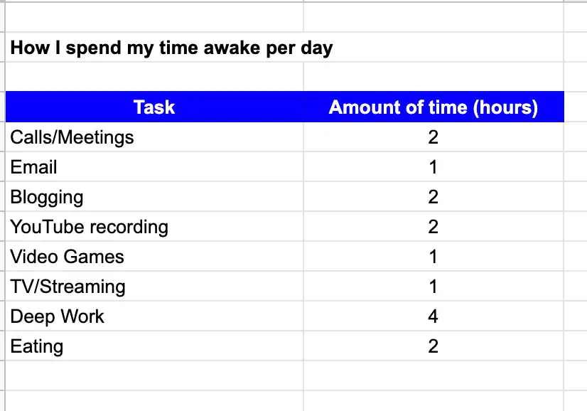
Before creating your pie chart, a data source is required. This may be school grades or sports results with their frequency. The key is that you need some data from which Google Sheets can generate a pie chart.

So let’s get started creating a pie chart in Google Sheets!

Step by Step Guide to Create a Pie Chart on Google Sheets

The following are detailed steps of how to create a pie chart on Google Sheets.

Step 1: Select the Data You Want to Use for Your Pie Chart

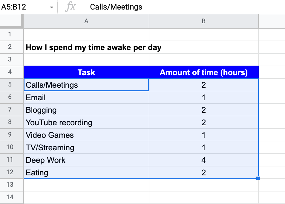
First, you should select the data to be used to generate the pie chart by left-clicking and dragging your mouse across the data you want to use as shown in the screenshot above.

Step 2: Go to Insert -> Chart in the Main Menu

In the main menu, go to Insert -> Chart, you have the option of creating a chart from the selected data. Select a pie chart from “Graph type” in the graph editor displayed on the right side of the spreadsheet.

Step 3: Generate a Pie Chart

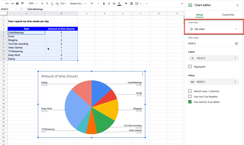
Depending on the context, Google Sheets inserts a different diagram as a suggestion. If the pie chart is not inserted initially, you can use the “Chart Type” option in the “Chart Editor” panel to convert the chart to a pie chart as shown in the screenshot above.

Looking to learn how to use conditional formatting in Google Sheets? You have to check out our Ultimate Guide to Conditional Formatting in Google Sheets.

Formatting a Pie Chart in Google Sheets

Now that you have generated your pie chart, there is a good chance you want to edit it in some way. So let’s go over the editing option available in Google Sheets for editing a pie chart.

Select Styles/Design Templates

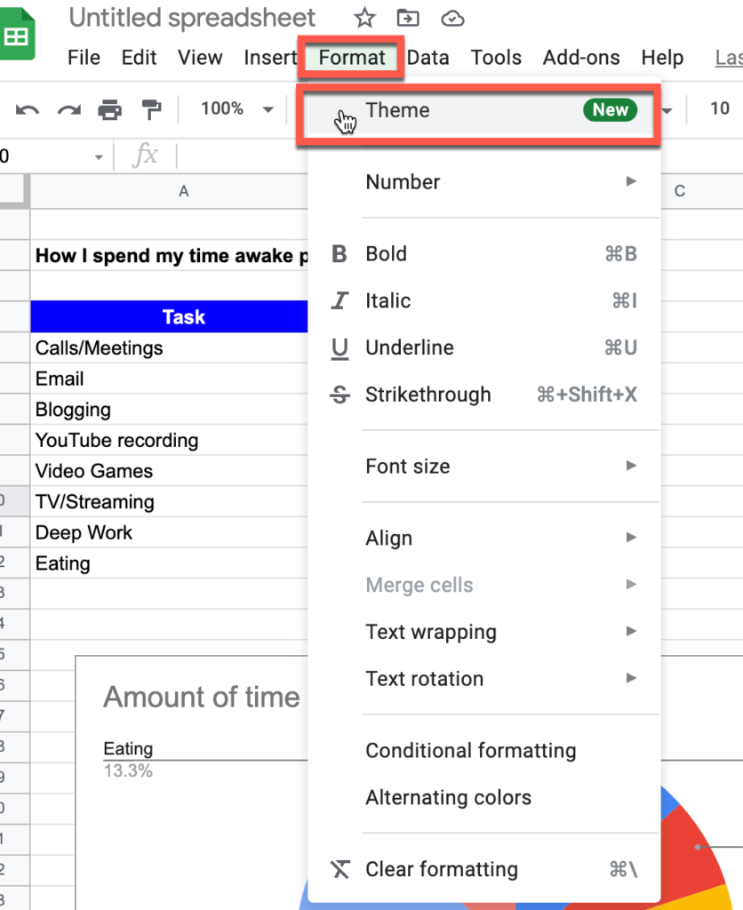
Sheets already has some pretty well-preformatted pie chart design templates. However, these are limited to basic formattings such as colors and text.

You can find these templates in the menu item “Format” and the sub-item “Design.”

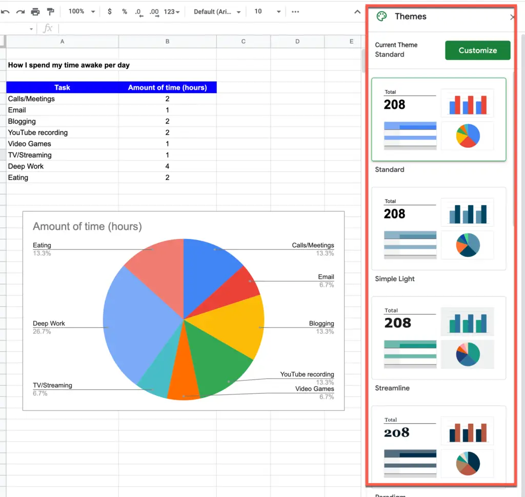
As you can see from the screenshot above, Google Sheets provides several options for themes you can use for your spreadsheet and pie chart.

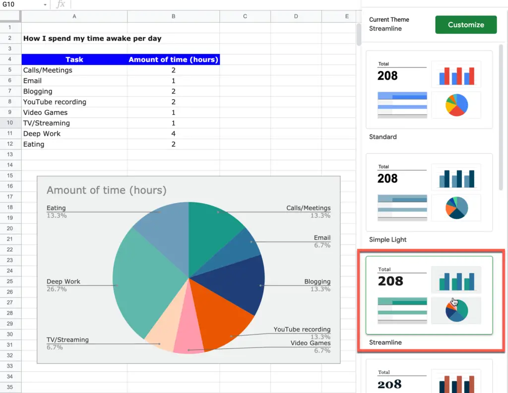
Simply click on the theme you want to use and the theme will change accordingly as you can see in the screenshot above.

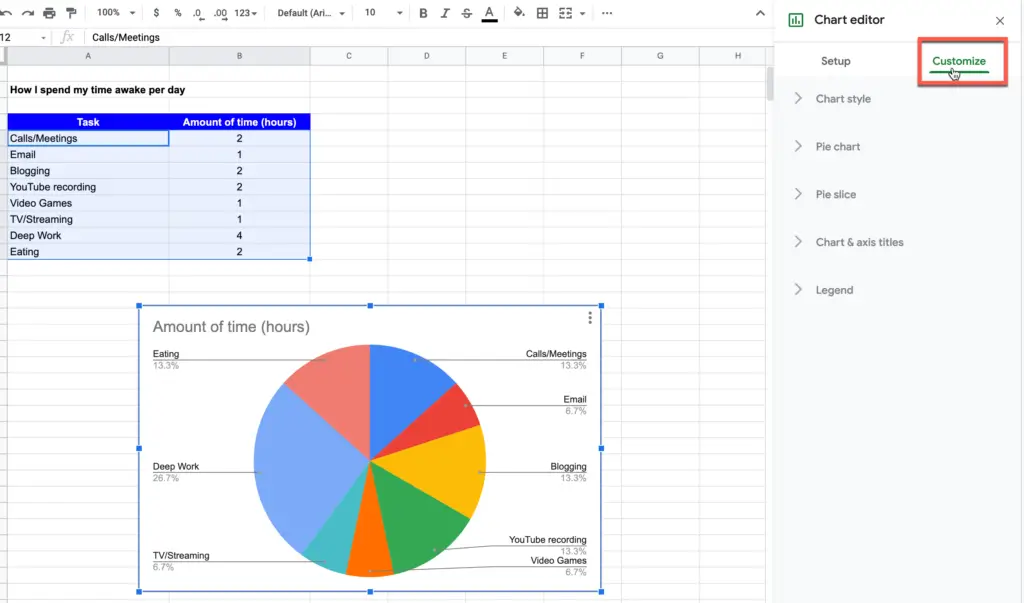
If changes are necessary, you can do this via the “Customize” tab of the “Chart Editor.” If you don’t select a design template, you can work on changes manually.

Format Title

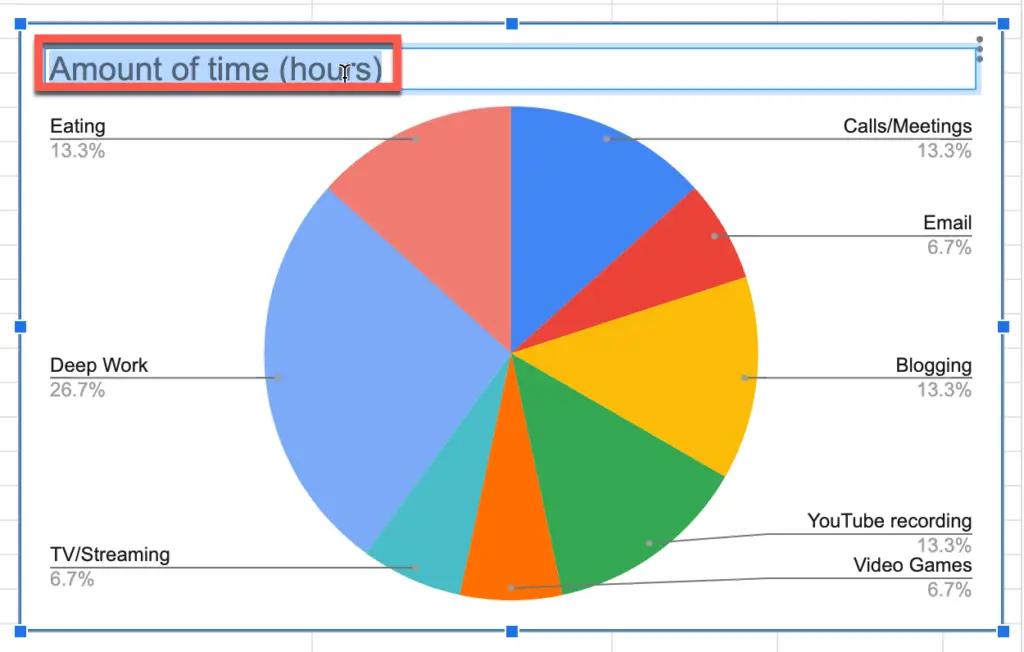
Since the title of the pie chart is composed of the column headings by default, you may want to change it.

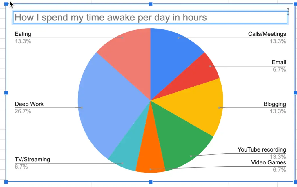
Double-click on the current title to select it. Press the backspace key to delete it and type in your new title as shown in the screenshot above.

Changing the color of a specific pie slice in Google Sheets

While Google Sheets come with excellent themes, you may want to change the color of a specific pie “slice”.

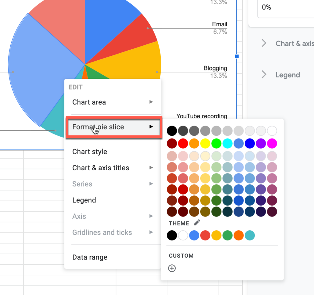
To do this, double-click to select the respective “piece of cake,” right-click and select “Format pie slice” from the available options. Then, choose an appropriate fill color.

Your pie slice should now be in the color you selected as shown in the screenshot above. This can be repeated for each part of the pie chart as needed.

Creating an Inner Circle to a Pie Chart in Google Sheets

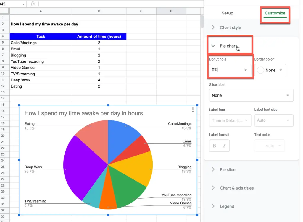
You can also make a donut out of the cake by adding an inner circle. To create a donut hole inside your pie chart, do the following:

1. Right-click on your pie chart
2. Select “Chart Style” from the available options to bring up the Chart Editor panel
3. Click on the “Customize” tab
4. Click on the “Pie Chart” dropdown to open up the pie chart options
5. Click on the “Donut Hole” dropdown and select the size percentage you want

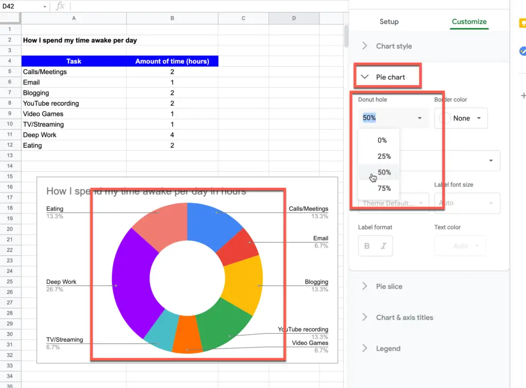
You can format this in 25% steps. You can also choose 50%. The option is in the “Pie chart” subsection of the “Customize” area of ​​the diagram editor as shown in the screenshot above.

Customizing Pie Chart Labels in Google Sheets

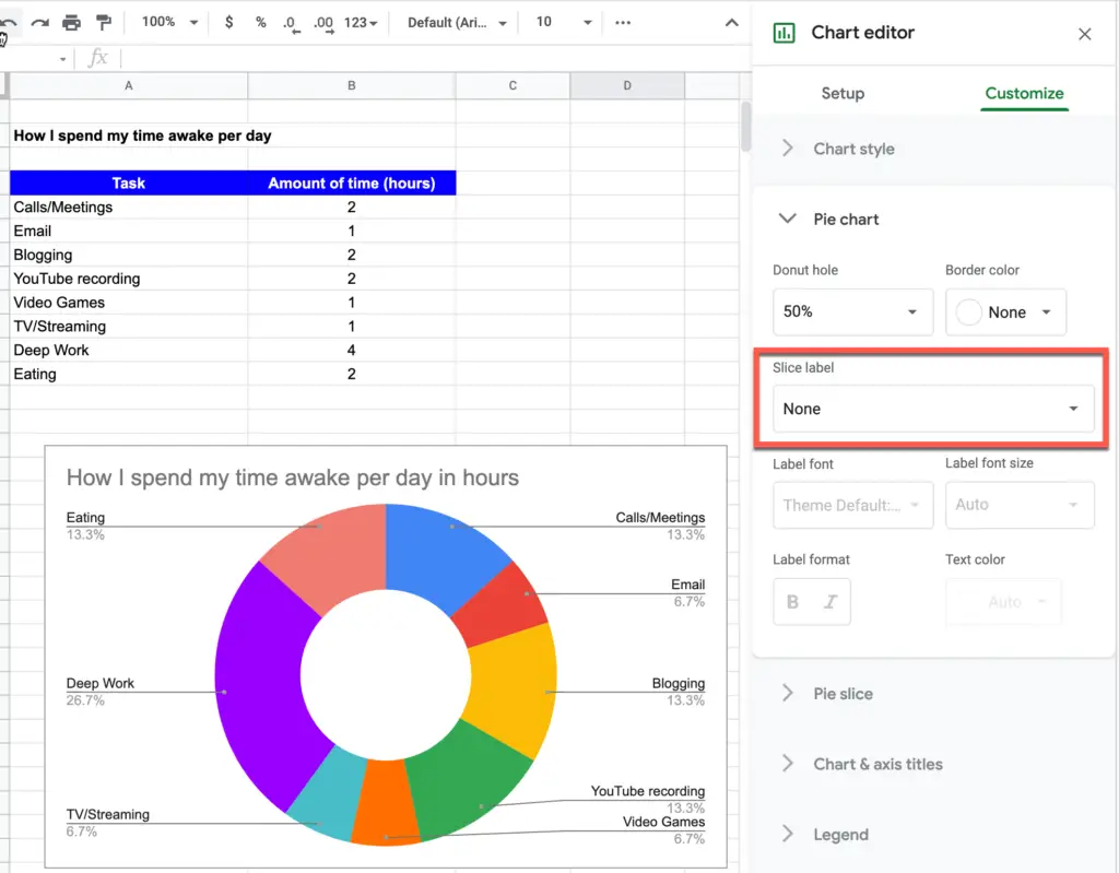
At the same time, you can provide each segment with a segment label. There are “Label,” “Value,” “Percent,” and “Value and Percentage.”

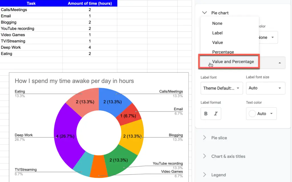
By choosing the latter, you will see the absolute and relative frequencies in each segment as shown in the screenshot above.

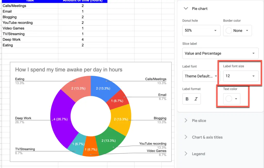
In addition, you can set the font color to white and reduce the font size a little if only partial segments are provided with frequencies.

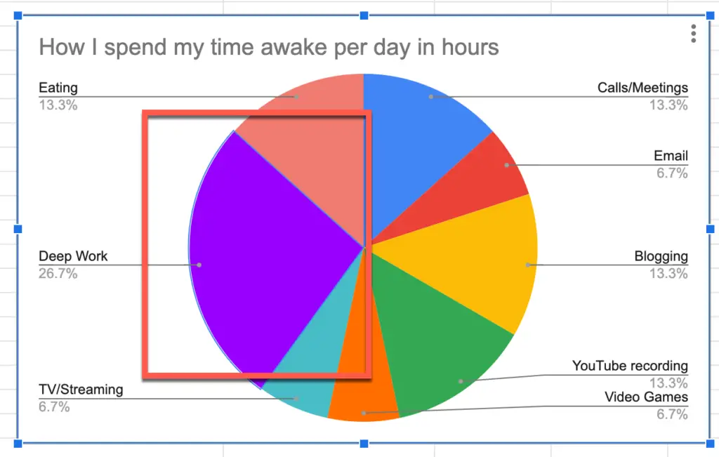
Changing the Distance to the Center (“Circle Explosion”)

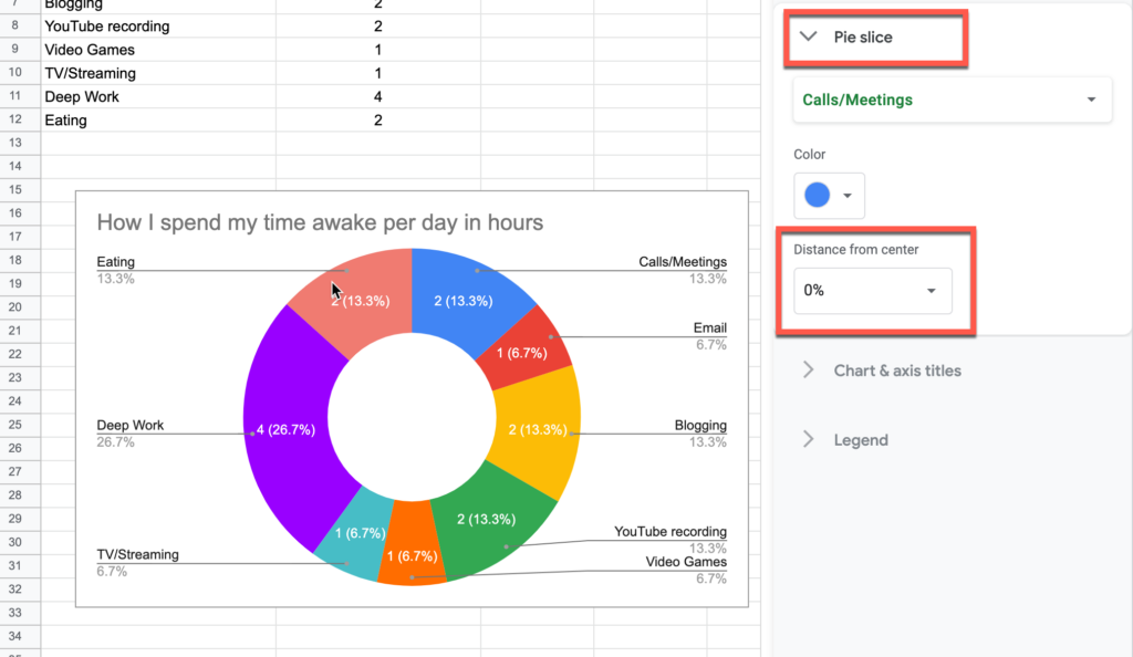
To emphasize a pie slice by offsetting it from the center of the circle in Google Sheets, do the following:

1. Double-click on the pie slice you want to emphasize to bring up the Chart Editor for that slice
2. Click on the “Customize” tab
3. Click on the “Pie slice” dropdown
4. Click on the “Distance from center” dropdown and select the offset percentage

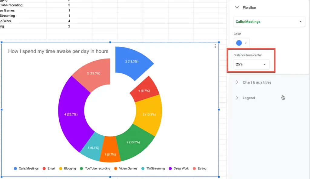
You should see your pie slice offset as shown in the screenshot above.

Downloading a Created Pie Chart

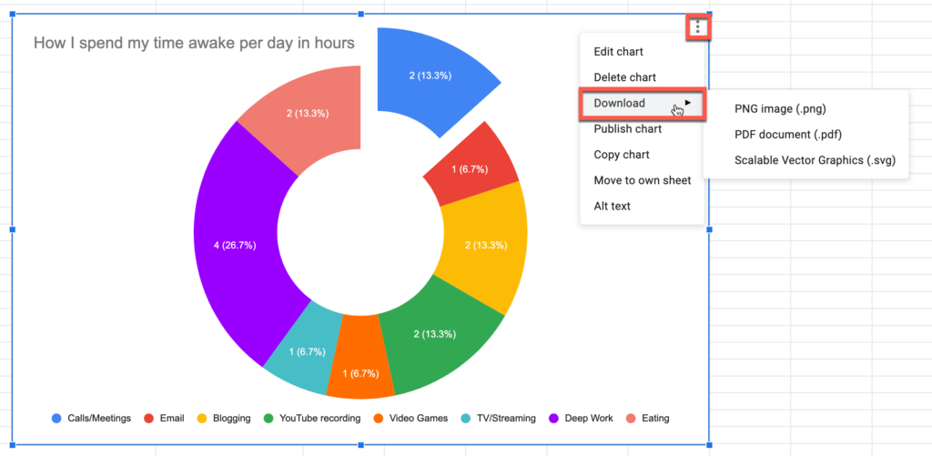
You can download your pie chart as an image file or PDF. To download your pie chart in Google Sheets, do the following:

1. Click on the pie chart
2. Click on the vertical ellipsis button in the upper-right corner of the pie chart
3. Select “Download” from the option
4. Select the file type you want from the available options

Publishing a Pie Chart

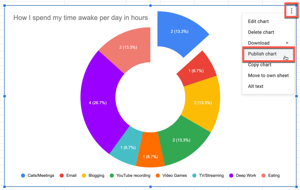
To publish your pie chart to the web in Google Sheets, do the following:

1. Click on the pie chart
2. Click on the vertical ellipsis button in the upper-right hand corner of the pie chart window
3. Select “Publish chart” from the available options
4. Click on either the “Link” or “Embed” tab based on your needs
5. Click the “Publish” button

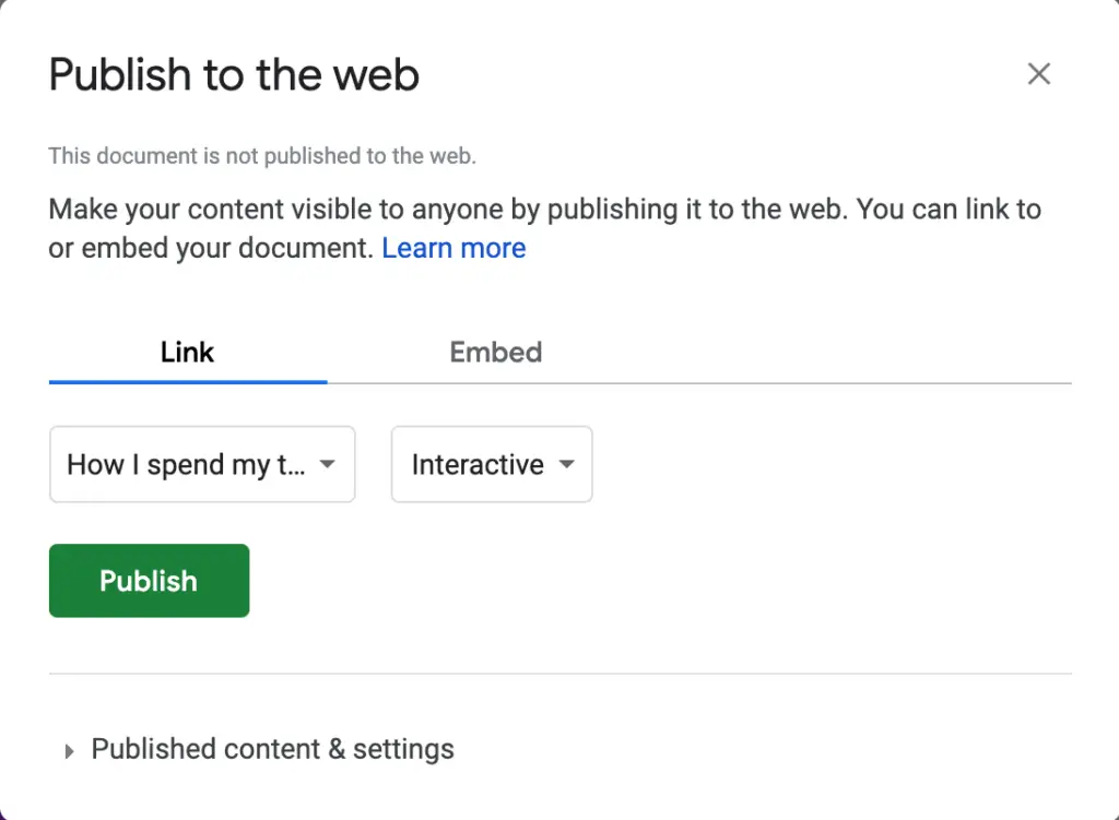
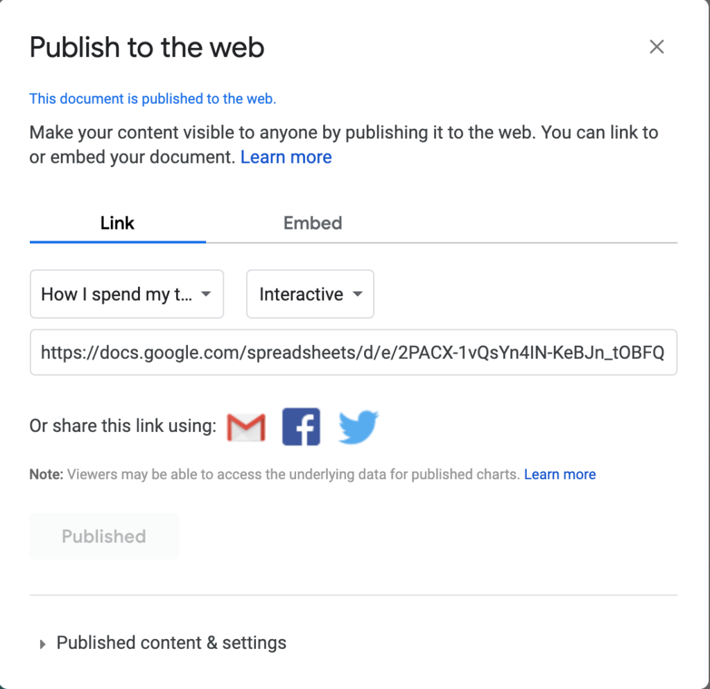
Your pie chart should now be published and accessible either via URL if you chose the “Link” option or as an embeddable code for your website via the “Embed” option

I hope this tutorial was helpful to you. Good luck!

Check out our Resources Page

Check out our resources page for the products and services we use every day to get things done or make our lives a little easier at the link below:

Link to the resources page

Want More Tips and Tricks? Subscribe to our Newsletter!

If you haven’t already subscribed, please subscribe to The Productive Engineer newsletter. It is filled with tips and tricks on how to get the most out of the productivity apps you use every day. We hate spam as much as you do and promise only to send you stuff we think will help you get things done.

We have a YouTube channel now and we are working hard to fill it with tips, tricks, how-tos, and tutorials. Click the link below to check it out!

link to our YouTube page

Can’t Remember Your Passwords? You Need 1Password!

Do you use the same password for multiple sites? Do you have trouble remembering all your passwords? You should try 1Password! 1Password is secure and allows you to log in to sites and fill out forms securely with a single click. I use 1Password for all my passwords and it really makes managing all my passwords simple.

For more information on 1Password and to get a 14-day free trial, go to 1Password at the link below:

1Password – The world’s most-loved password manager