Conditional Formatting in Google Sheets: The Ultimate Guide

Spreadsheets have been an integral part of business operations for decades now. Conditional formatting is a helpful tool to any spreadsheet, though it can be intimidating if you are unfamiliar with it. Let’s take the mystery out of using conditional formatting to make your spreadsheets in Google Sheets easier to read.

What is Conditional Formatting?

Conditional formatting in Google Sheets allows the editor of a spreadsheet to set formatting rules based on the content entered into the cells. If the information in the cell(s) matches the criteria, it will be formatted in one way; if it does not, Google Sheets can format it differently.

Some examples of this might be a spreadsheet keep keeping track of sales for the month. Should sales fall below a certain margin, the color of the cell may turn red. If the sales should spike above a particular margin call, the cell may turn green.

This type of Conditional Formatting has many functions. Not only can it allow the author to control how information is presented in the spreadsheet, but it can also allow for quicker dissemination of information. Because of the formatting differences, conditional formatting will quickly draw your eye to the information contained in the cells. The enhanced formatting will make it easier to notice and read important information at a glance.

What Criteria can I use to Conditionally Format cells/rows in Google Sheets?

Several preset formulas are available for you to use for conditional formatting. They cover the more basic functions that one would use to format their spreadsheet for easier reading and data recognition.

Enclosed below is a table showing all the possible criteria you can use to conditionally format cells in Google Sheets:

Criteria	Description
is empty	applies formatting if the cell(s) is empty
is not empty	applies formatting if the cell(s) is not empty (i.e. contains a value)
Text contains	applies formatting if the type is text and contains a specific character or string of characters
Text does not contain	applies formatting if the type is text and does not contain a specific character or string of characters
Text starts with	applies formatting if the text starts with a specific character(s)
Text ends with	applies formatting if the text ends with a specific character(s)
Text is exactly	applies formatting if the text exactly matches the character(s)
Date is	applies formatting if the date in the cell matches a specific date
Date is before	applies formatting if the date in the cell is before a specific date
Date is after	applies formatting if the date in the cell is after a specific date
Greater than	applies formatting if the value in the cell is greater than a defined value
Greater than or equal to	applies formatting if the value in the cell is greater than or equal to a defined value
Less than	applies formatting if the value in the cell is less than a defined value
Less than or equal to	applies formatting if the value in the cell is less than or equal to a defined value
is equal to	applies formatting if the value in the cell is equal to a defined value
is not equal to	applies formatting if the value in the cell is not equal to a defined value
is between	applies formatting if the value in the cell is within a defined range of values
is not between	applies formatting if the value in the cell is not within a defined range of values
custom formula is	applies formatting based a custom defined formula created by the user

The final possibility in the “Format Cell if” drop-down menu is the Custom Formula. This is the area that will allow you to personalize your spreadsheet formatting to fit your specific needs. Using a formula approach, you can customize the Conditional Formatting to highlight information that might not be covered in the preset formatting functions.

How to Access the Conditional Formatting Options in Google Sheets

1.  Open Google sheets
2.  Select the range of cells you want to format.
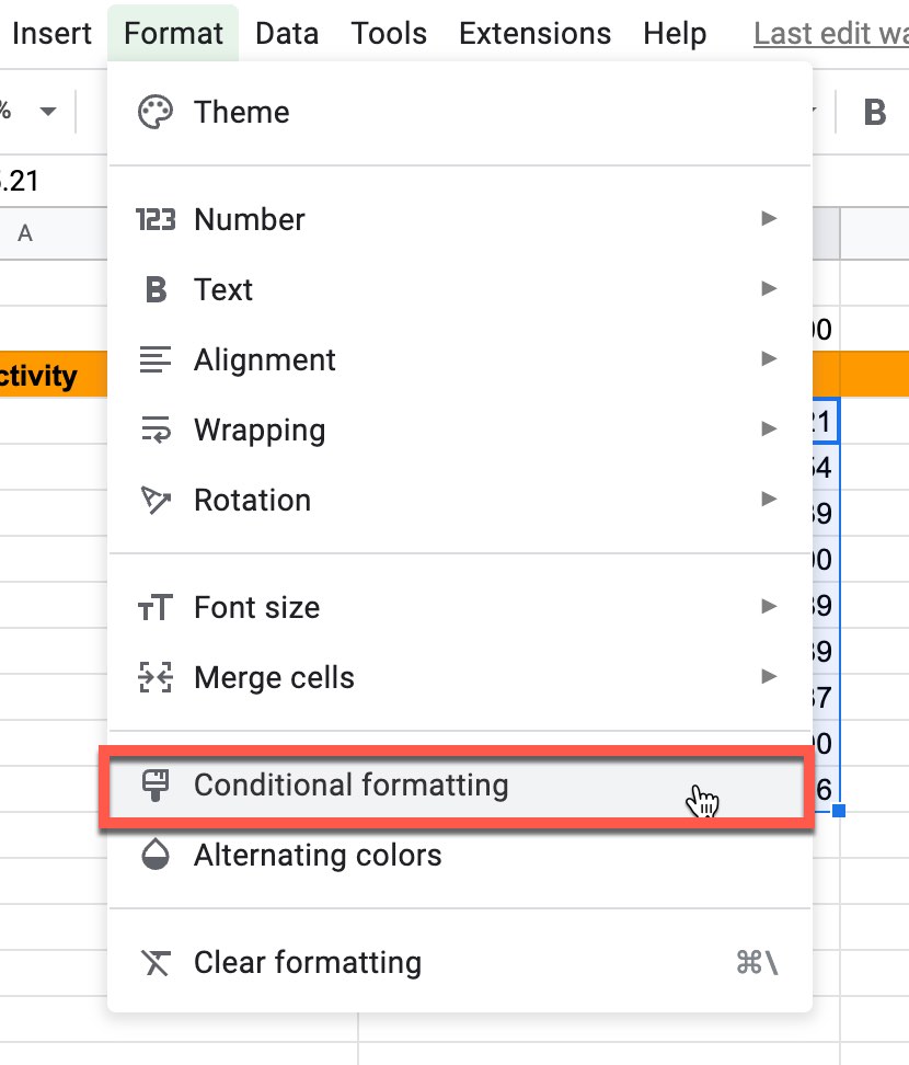
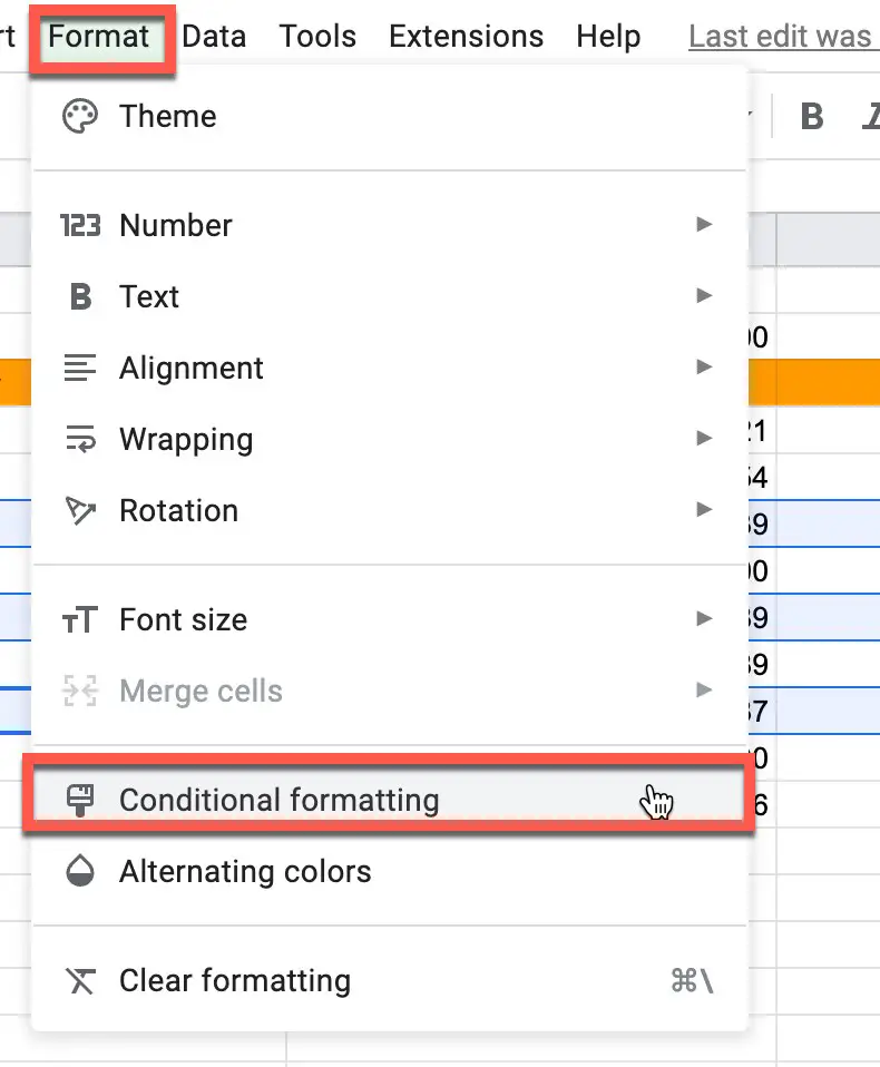
3. In the main menu, select Format This will open a drop-down menu. Select Conditional Formatting

Open Google Sheets

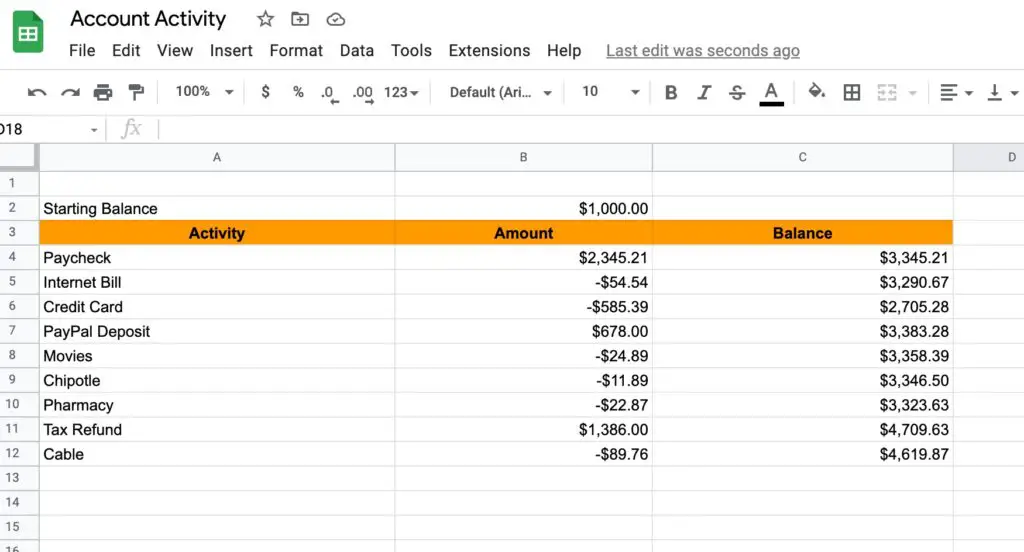
Go to https://sheets.google.com. Open up the spreadsheet that you want to use conditional formatting in. In our tutorial, we will use this simple account tracking spreadsheet.

Select the Range of Cells You Want to Format

Click and drag to select the cell(s) you want to conditionally format.

In the Main Menu, Go to Format -> Conditional Formatting

As shown in the screenshot above, in the main menu, go to Format -> Conditional Formatting.

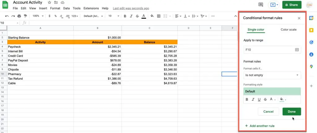
You should now see the conditional formatting rules as shown in the screenshot above.

How to change cell color based on the value of cells in Google Sheets.

One of the most common things you will want to do is to change the color of the cell in Google Sheets based on the value of the cell.

Listed below are the steps required to change the color of a cell in Google Sheets based on the value of the cell:

1. Select the cell(s) you want to conditionally format
2. Select Format -> Conditional Format  in the main menu
3. Under Format Rules, click the drop-down box and select the criteria you want for the list of options
4. In the Formatting Styles, select the style of formatting you would like if the conditions were met.
5. Click Done for changes to take effect.

To illustrate how to do this, we will use our account activity spreadsheet and change the color of the cell to green for any value greater than zero.

Select the cell(s) you want to conditionally format

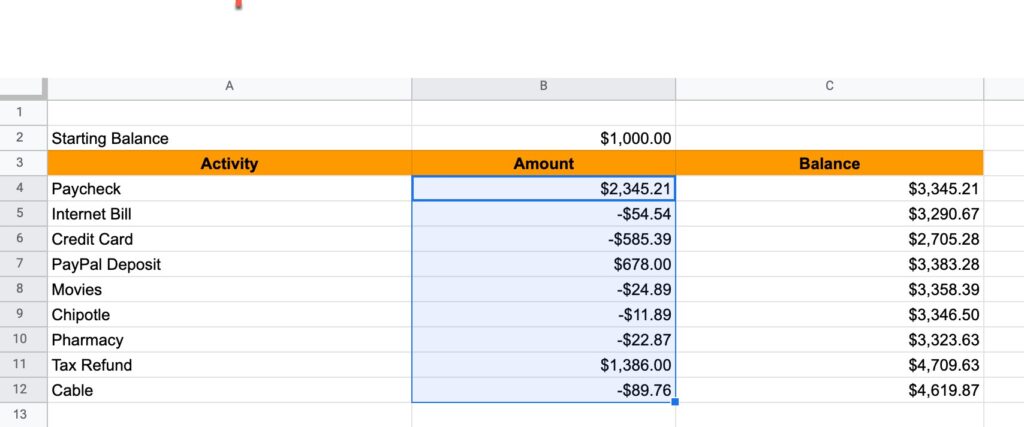
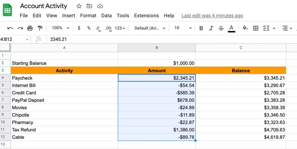
First thing we need to do is to select the cells we want to evaluate and conditionally format. Click and drag your mouse across the cells you want to include in the evaluation.

Select Format -> Conditional Formatting from the main menu

Once you have selected your cells, go to Format -> Conditional Formatting in the main menu to bring up the Conditional Formatting Rules menu.

Under Format Rules, click the drop-down box and select the criteria you want for the list of options

You should see a section of the Conditional Format Rules titled “Format Rules” with a drop-down menu. Click on the drop-down menu in this section to bring up the available options. For our example, we are looking to conditional format all values greater than zero so we will choose the “Greater than option as shown above.

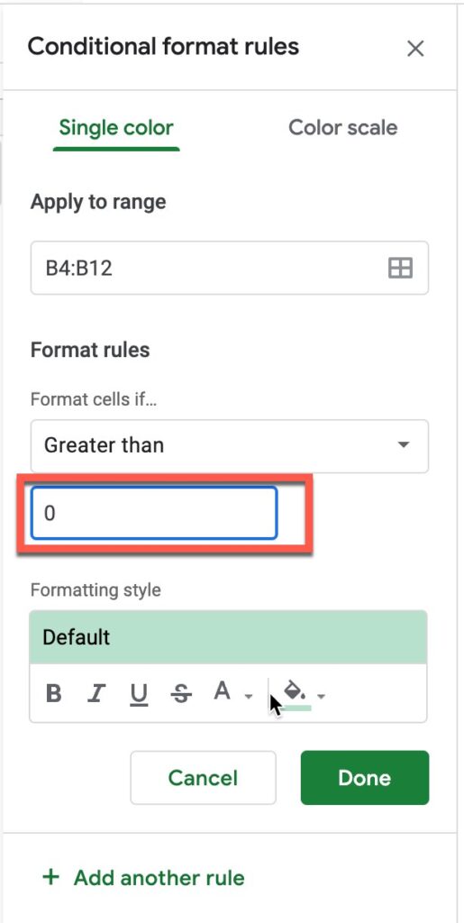
We need to fill in a value for the greater than option. As we want to format all values greater than zero, we entered zero as shown in the screenshot above.

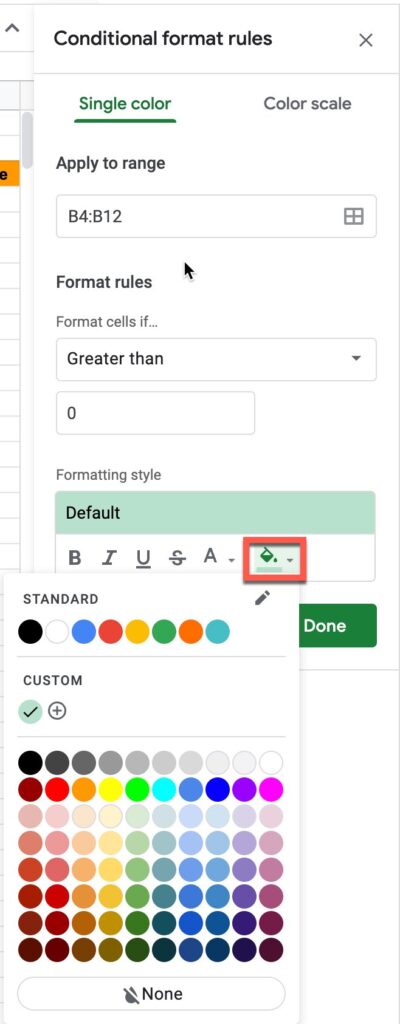
Next, you can set the fill color in the “Formatting style” sub-section of the “Format Rules” section as shown above. Click on the “paint bucket” button to bring up the color palette as shown above. Click on the color you want to use as your fill color.

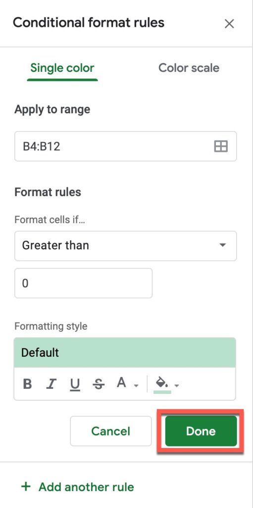
For our example, we chose green. Click the “Done” button as shown above to save your conditional formatting rule.

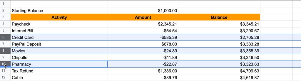
As you can see, our rule now shows up in the “Conditional format rules” section and all of the cells we selected that are greater than zero as now shaded green.

How to Conditionally Format An Entire Row in Google Sheets

1. Click on the row number for that row
2. In the main menu, go to Format -> Conditional formatting  
3. Under “Format rules”, click on the “Format cells if…” drop-down menu
4. Select the condition option you want
5. Under “Formatting style”, select the formating you want to apply
6. Click the “Done” button to save and apply your conditional formatting rule

Let’s dive deeper into each of these steps.

Click on the Row Number

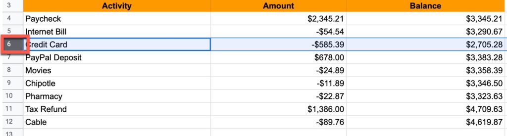
The first thing we want to do is select the row we want to conditionally format. To do this, simply click on the row number of the row as shown in the screenshot above. This will select all the cells in the row.

If you want to select multiple rows, hold down the Command key on Mac or the Windows key on Windows and click each row number you want to select.

In the Main Menu, go to Format -> Conditional formatting  

Next, in the main menu, go to Format -> Conditional Formatting as shown in the screenshot above.

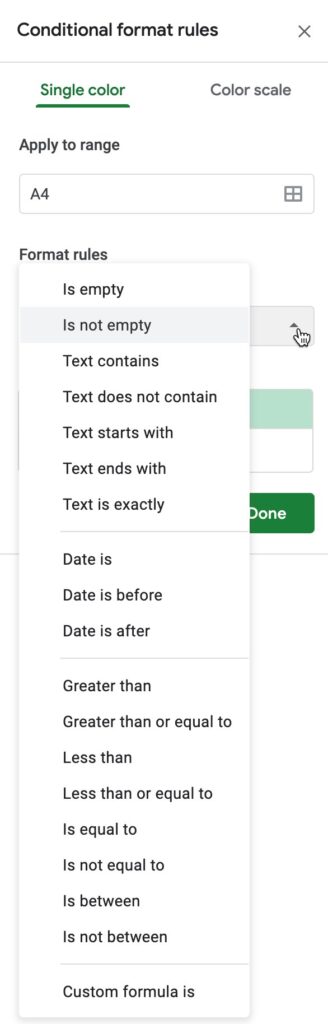
Under “Format rules“, click on the “Format cells if…” drop-down menu

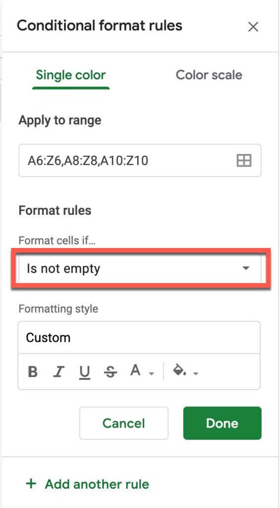
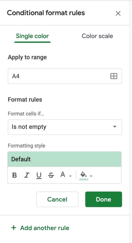
You should now see the “Conditional format rules” section as shown above. Click the drop-down menu underneath the “Format cells if…” subheading.

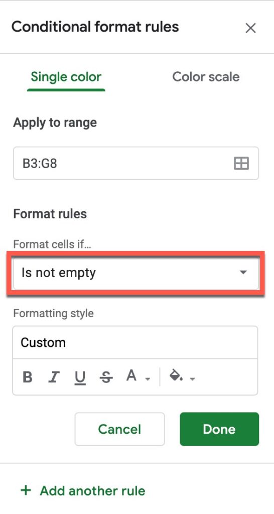
Select the Condition Option You Want

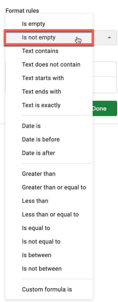
Select the condition you want from the available options. For our example, we will conditionally format all cells in our selected rows that are not empty so we will select “is not empty” as shown above.

Under “Formatting style“, Select the Formatting You Want to Apply

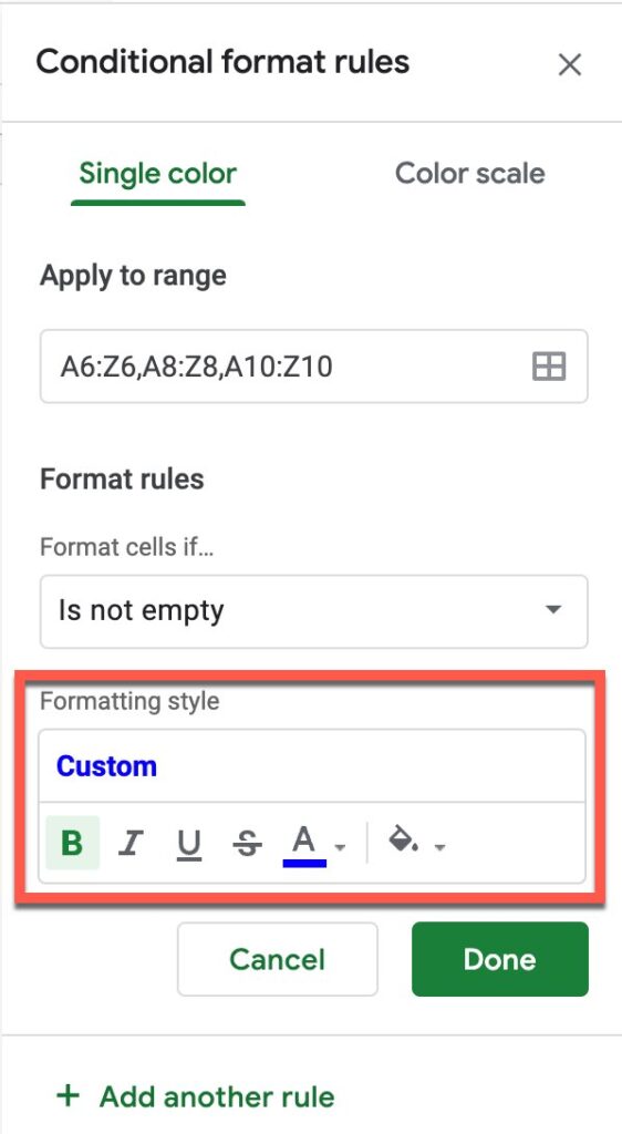
Next, apply the formatting you want to the cells that fit your conditional logic. For our example, we will bold the text and color the text blue. So we click the “B” button to bold the text and the “A” button and select blue from the color options as shown in the screenshot above.

Click the “Done” Button to Save and Apply Your Conditional Formatting Rule

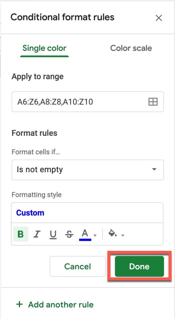
Once you have the conditional logic and formatting setup, click the “Done” button to save and apply your conditional formatting.

Your cells should now show the conditional formatting you applied.

How to Use Multiple Conditional Formatting Rules in Google Sheets

It is very common to have more than one Conditional Formatting Rule for one spreadsheet, even for one range of cells. It is possible to group more than one function per range of cells.

Enclosed below are the steps required to apply multiple conditioning formatting rules to a group of cells in Google Sheets:

1. Select the cells you want to format
2. Go to “Format” and Select “Conditional formatting”
3. Go to the “Format cells if…” Section and Click on the Drop-down Menu
4. Select the Condition You Want in the “Format cells if…” option
5. Set Your Condition Parameters if Necessary
6. Click “+ Add another rule” to Create a Second Conditional Formatting Rule
7. Select and Configure the Condition Criteria
8. Configure the Conditional Statement and Formatting Style and Click “Done” to Save
9. Repeat the Prior Steps for each New Rule You Want to Add

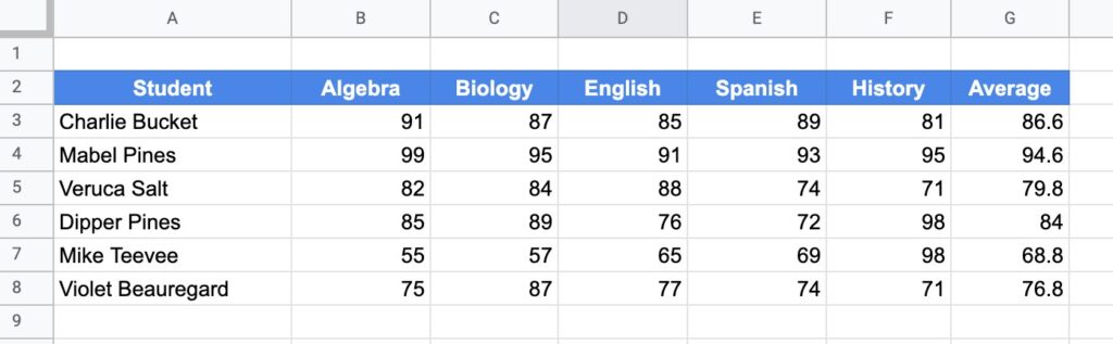
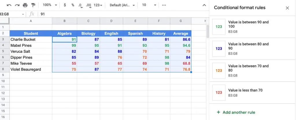
Here is a grade spreadsheet in Google Sheets. We will use multiple conditional formatting rules to assign specific colors based on the values in the cells we select.

Select the Cells You Want to Format

The first thing you want to do is to select the cells you want to apply your conditional formatting rules to. Click and drag your mouse across the cells you want to use as shown in the screenshot above.

Go to “Format” and Select “Conditional formatting”

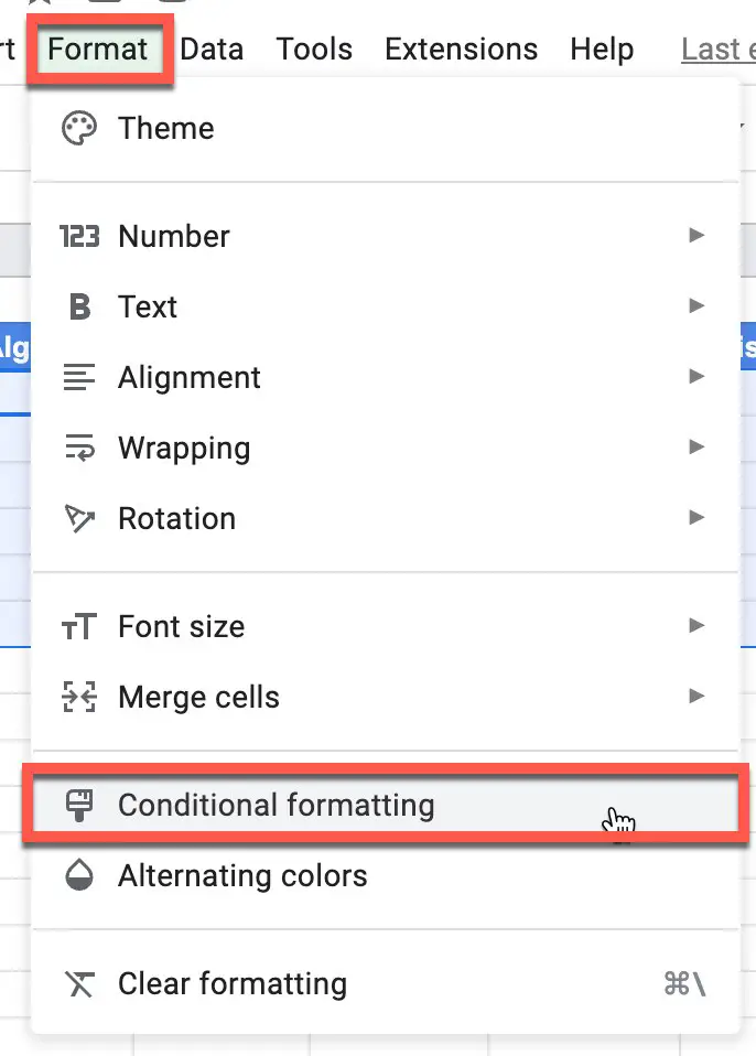
In the main menu, go to Format and select Conditional formatting from the available options as shown in the screenshot above.

Go to the “Format cells if…” Section and Click on the Drop-down Menu

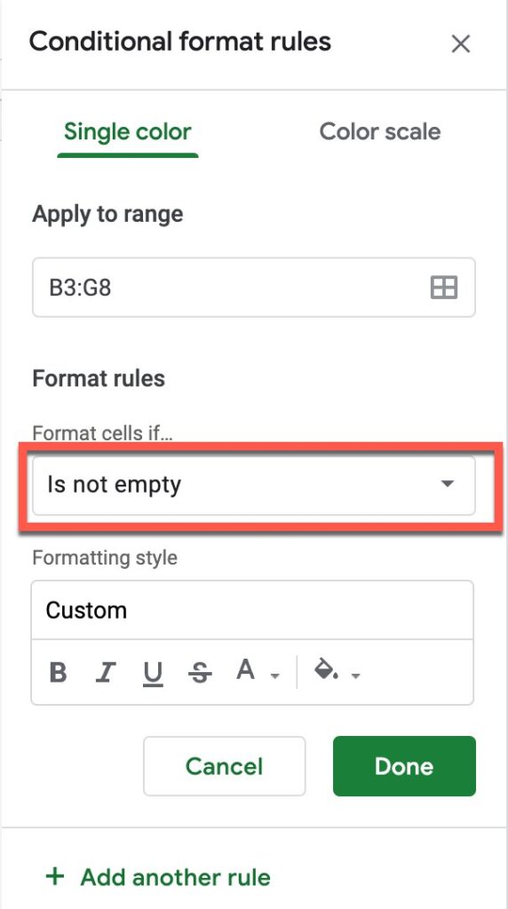
In the “Conditional formatting rules” menu, go to “Format cells if…” section and click on the drop-down menu as shown above.

Select the Condition You Want in the “Format cells if…” option

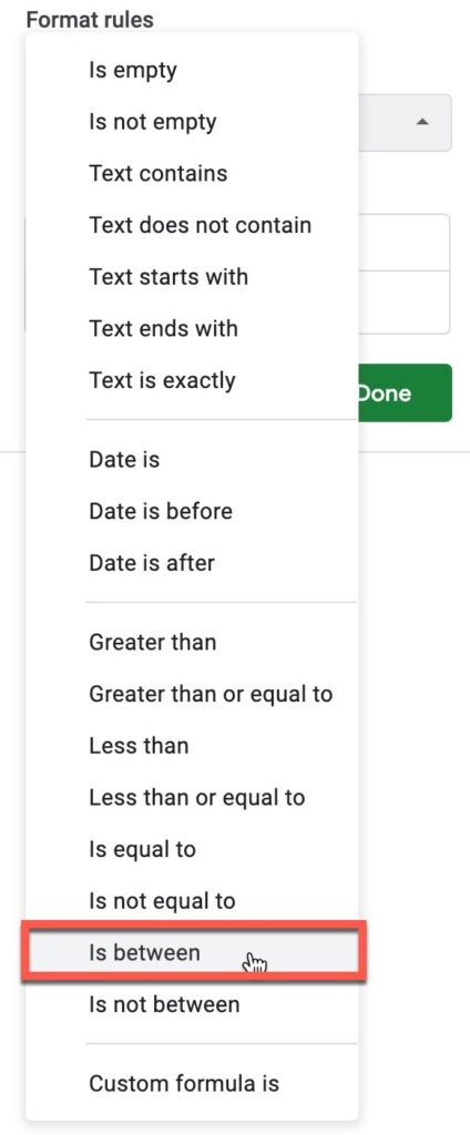
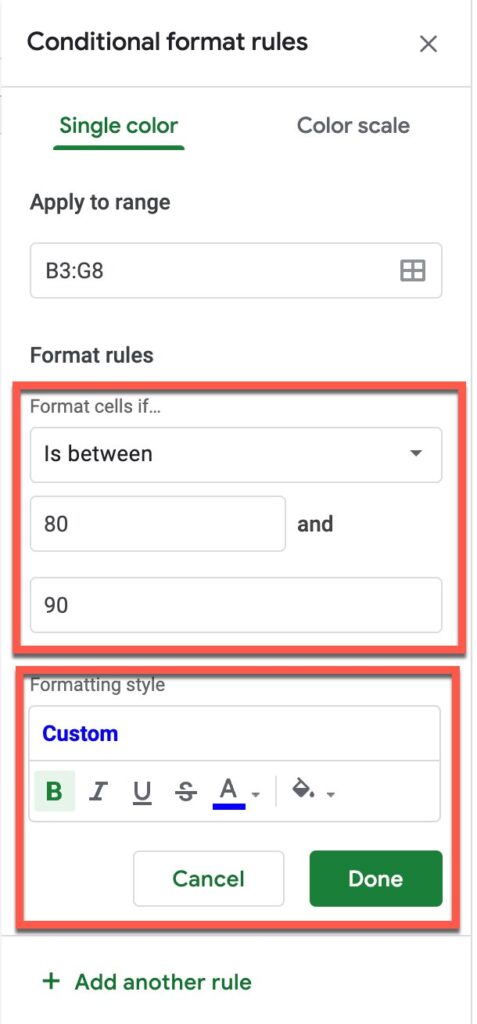
Once the drop-down menu appears as shown above, select the condition you want. In our example, we want to conditionally format cells whose values fall within a range of numbers so we will select “Is between” from the available options.

Set Your Condition Parameters if Necessary

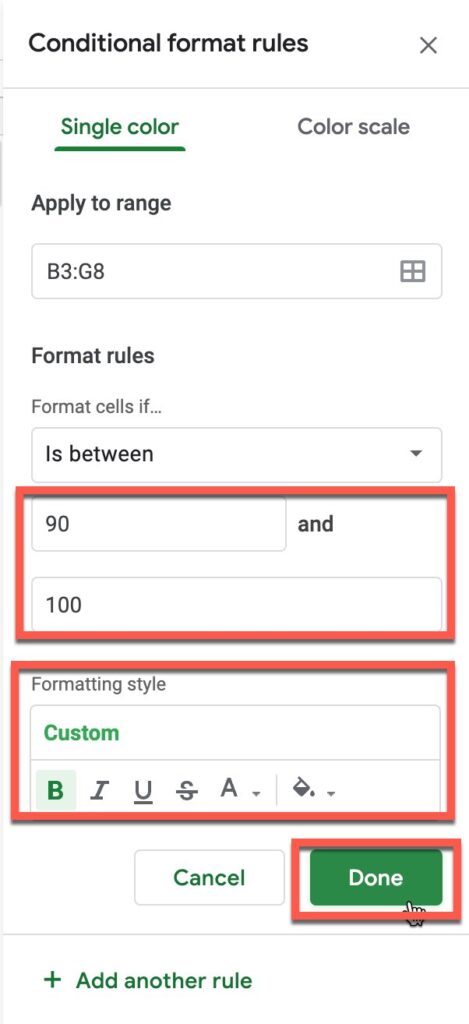
Some conditions require additional parameters or settings. In our example, we chose the “in-between” option to define a range of values. We need to add the range of values as shown above.

Once you have set your condition settings, configure the formatting in the “formatting style” section. We will set our example for this rule to be the following:

• Bold and set the text color to green for any selected cell that has a value between 90 and 100.

Once you have finished configuring the conditional and formatting, click the “Done” button to save and apply the conditional formatting rule.

Click “+ Add another rule” to Create a Second Conditional Formatting Rule

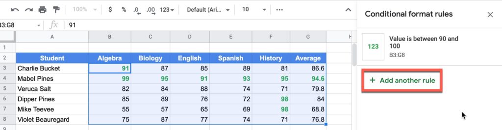
Now we need to add a second conditional formatting rule to our spreadsheet. In our example, we will add rules for the following grade ranges:

• 80-89
• 70-79
• 60-69

Each range will have its own rule. To get started adding an additional rule, select/reselect the cells and click the “+ Add another rule” button as shown in the screenshot above.

Select and Configure the Condition Criteria

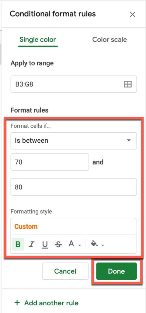
Like we did with the first conditional formatting rule, select the condition you want from the “Format cells if…” section. We will again choose “Is between” to define a second range of values that we can conditionally format.

Configure the Conditional Statement and Formatting Style and Click “Done” to Save

Configure the conditional logic and formatting style for your second conditional formatting rule. In our example, we are going to do the following:

• Bold and change the text color to blue any cell that have a value between 80 and 90

Once you have finished setting up the rule, click the “Done” button to apply and save the rule.

Repeat the Prior Steps for each New Rule You Want to Add

Repeat the prior steps for each of the new rules you want to add. I have enclosed the screenshots of each additional rule I added to our example spreadsheet

I sincerely hope that this tutorial has taken some of the mystery out of using Conditional Formatting to enhance your Google Sheets experience! Have fun with it!