How to Lock Formatting and Cells in Google Sheets - The Ultimate Guide

Google Sheets has seen a significant rise in its users over recent years as it continues to assert itself as a powerful and free alternative to Microsoft’s Excel. One issue that even power users come up against is how to lock the formatting of cells in Google Sheets.

How to Lock Formatting in Google Sheets

Formatting can be locked in Google Sheets by creating a protected range. However, this also means that the values of the cells in the range will not be editable. The only workaround to this is to use Google Apps Script to reapply the formats each time the spreadsheet is edited.

Understanding what Google Sheets features your use case requires you to use can seem a bit tricky. Keep reading to find out the best way to solve your formatting problem in Google Sheets.

How Do I Lock Cells in Google Sheets?

Protecting a range of cells (or even the entire sheet) allows you to prevent users from making changes to the cells and their values when working in Google Sheets — effectively ‘locking’ them. This is useful when you might want to keep the cells values and formats consistent while also allowing multiple users to access certain parts of your Google Sheets file.

The first thing you’ll need to ensure is that your user account has the right permission level for the file. Adding a protected range requires the permission level Editor or higher. You can check this by clicking the ‘Share’ button in the top right and finding your user email. If you can’t see the button, this means you do not have sufficient access.

In order to apply protection to cells in Google Sheets, you need to perform the following steps:

Select the cells you wish to protect
Select Data from the menu, and then Protected sheets and ranges
Ensure the right range is entered, and enter a description if desired
Click Set permissions
Select the users you wish to allow to edit the cells

Select the cells you wish to protect

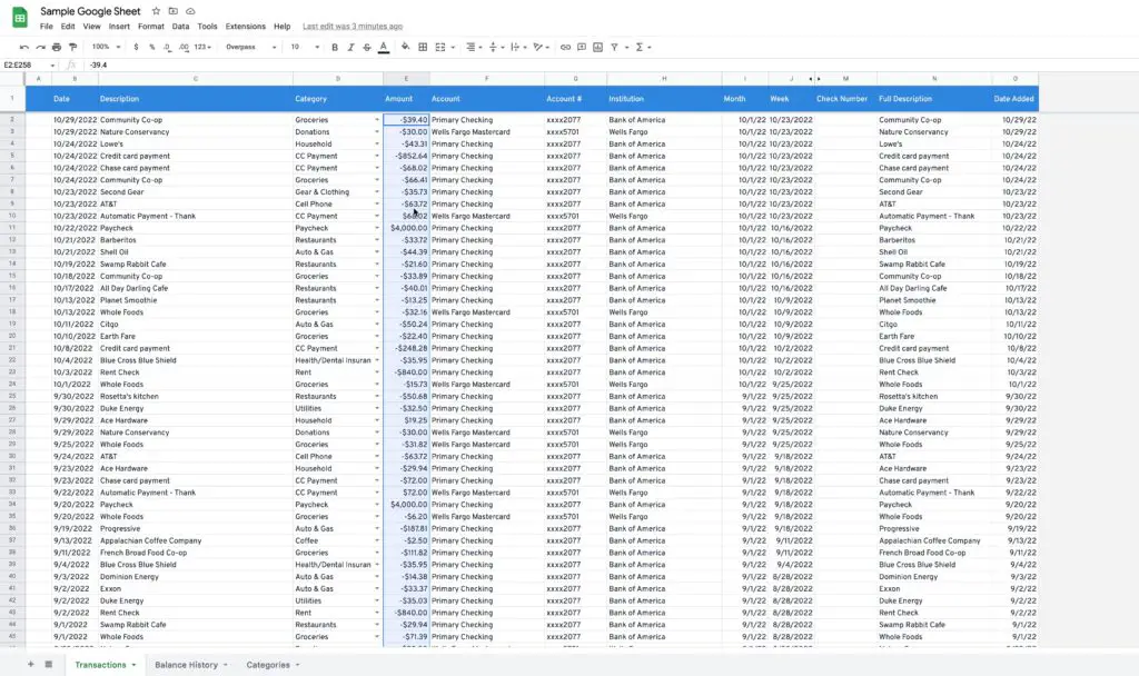
Select cells by clicking and dragging mouse across cells — Select cells by clicking and dragging the mouse across cells

The first step is to select the cells you want to protect by clicking and dragging your mouse across the cells you want to protect as shown in the screenshot above.

Select Data from the menu, and then Protected sheets and ranges

In main menu, go to Data -> Protect sheets and ranges — In the main menu, go to Data -> Protect sheets and ranges

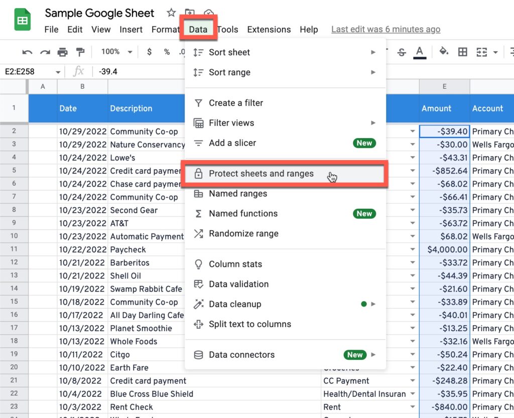
Next, in the main menu, go to Data -> Protect sheets and ranges as shown in the screenshot above.

Ensure the right range is entered, and enter a description if desired

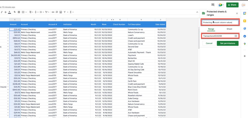
Make sure that you label your protected range and that you have the correct cells selected

You should see a new panel on the right-hand side of your Google Sheets window like the one shown above. Enter a description for your protected range and make sure that you have the appropriate cells selected in the “Range” field.

Click Set permissions

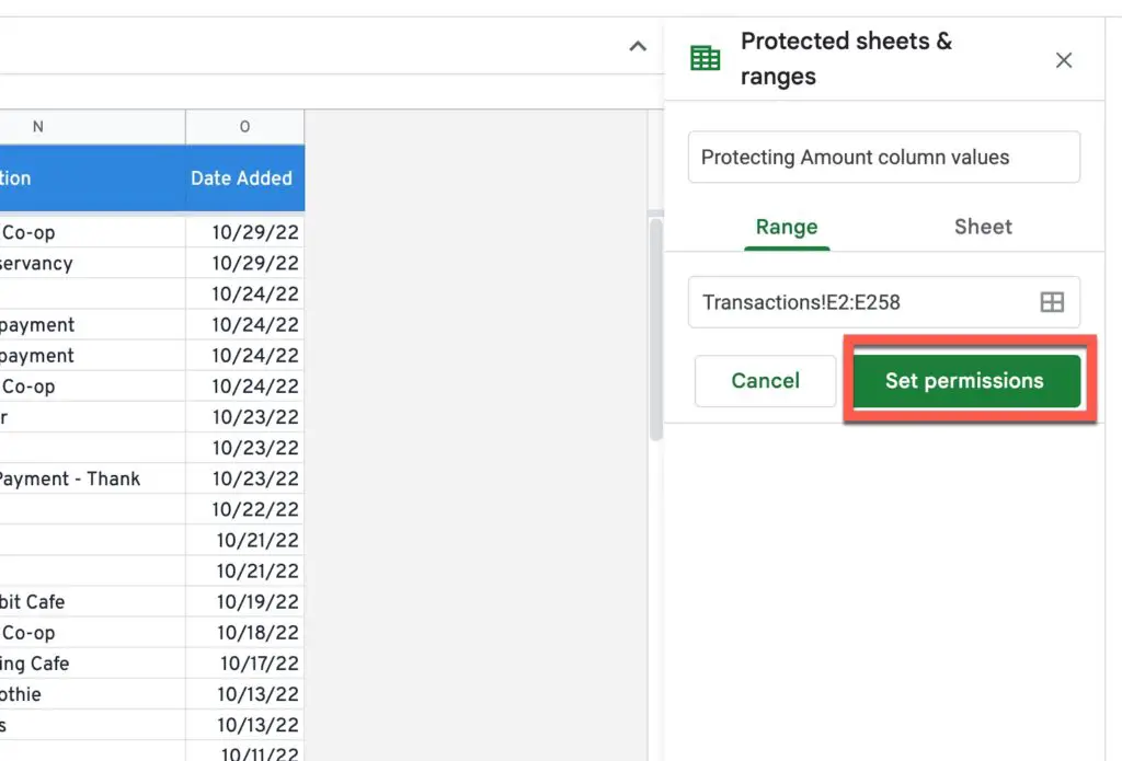
Click the "Set permissions" button — Click the “Set permissions” button

Once you have verified that you have selected the cells you want, click on the “Set permissions” button as shown in the screenshot above.

Select the users you wish to allow to edit the cells

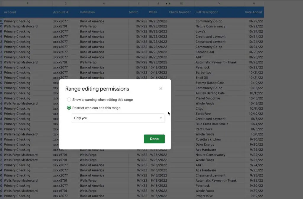
Range editing permissions pop-up dialog box

You should now see the “Range editing permissions” dialog box as shown above. Click on the drop-down menu option under the “Restrict who can edit this range” option.

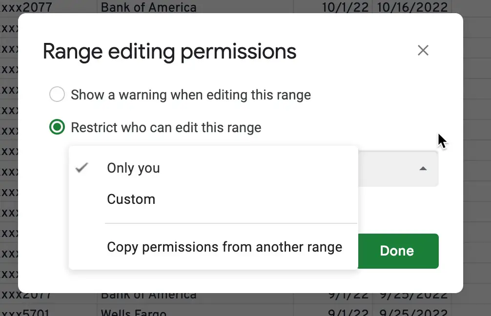
Range editing permission options in Google Sheets

You should see the following options as shown above:

Only you (default)
Custom
Copy permissions from another range

If you want to ensure that only you can edit the range, leave the “Only you” option selected and click the “Done” button.

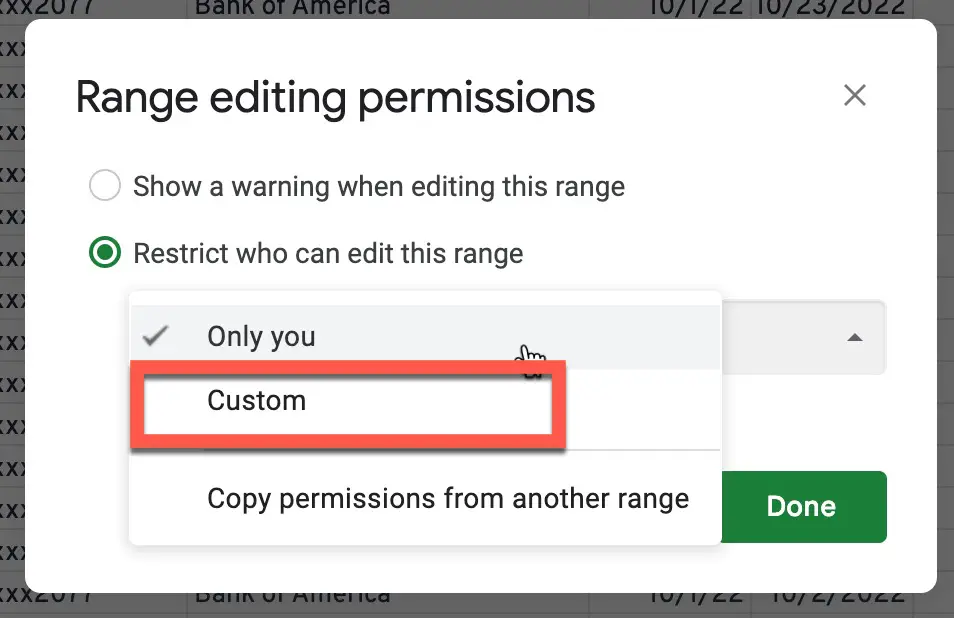
Choose "Custon" to add more people who can edit the cells in the range — Choose “Custon” to add more people who can edit the cells in the range

If you want other people you select to also be able to edit the protected cells, choose “Custom” from the drop-down menu as shown in the screenshot above.

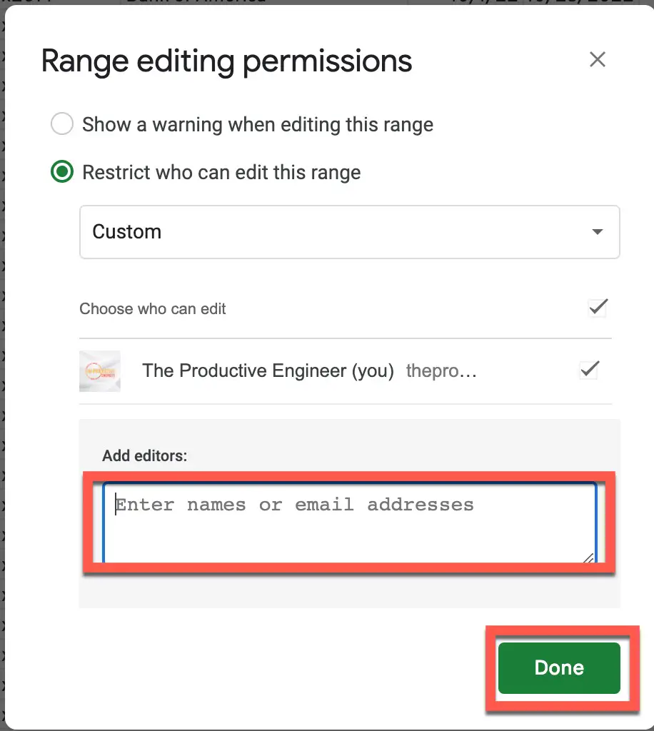
enter the names or email addresses of people you want to grant edit access to

You should now see the dialog box shown above. Under “Add Editors”, enter the names or email addresses of the people you want to be able to edit the range and click the “Done” button.

Error message that unauthorized users will see when they attempt to edit cells in range

Following this process will create a ‘protected range,’ meaning that only those users you have selected are able to edit those cells.

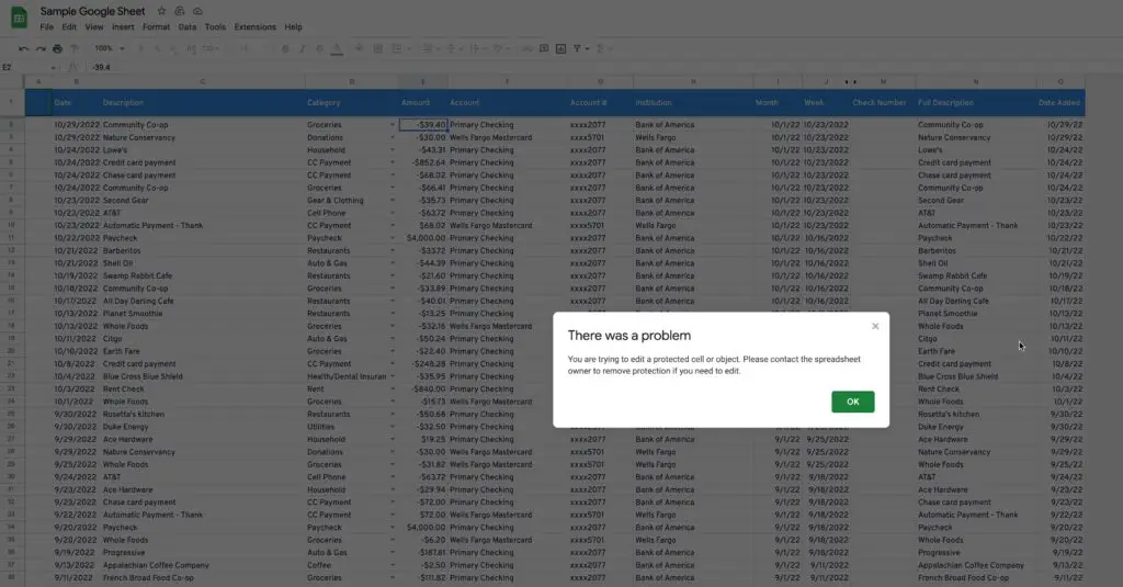
It is important to note that this protection restricts users from taking a number of actions relating to cells within the protected range. The users cannot:

Change the formatting of the cell
Change the value of the cell
Make changes impacting the row and column (e.g., applying a filter)

How Do I Edit or Remove a Protected Range in Google Sheets?

It is very straightforward to make changes or remove a protected range in Google Sheets. You first need to ensure that you have the required permissions to be able to do so.

Making changes to protected ranges (and being able to see the protected ranges at all) is dependent upon whether your user account has an Editor permission level or above. If you have either a Viewer or Commenter permission level, you will not be able to make the changes.

To remove or edit the permissions on a protected range in Google Sheets, there are a few simple steps to follow:

Select Data from the menu, and then Protected sheets and ranges
Click on the range entry you wish to change or delete
Then:
- To delete the range, click the trash can icon
- To edit the range, simply edit the elements, and click Done

Select Data from the menu, and then Protected sheets and ranges

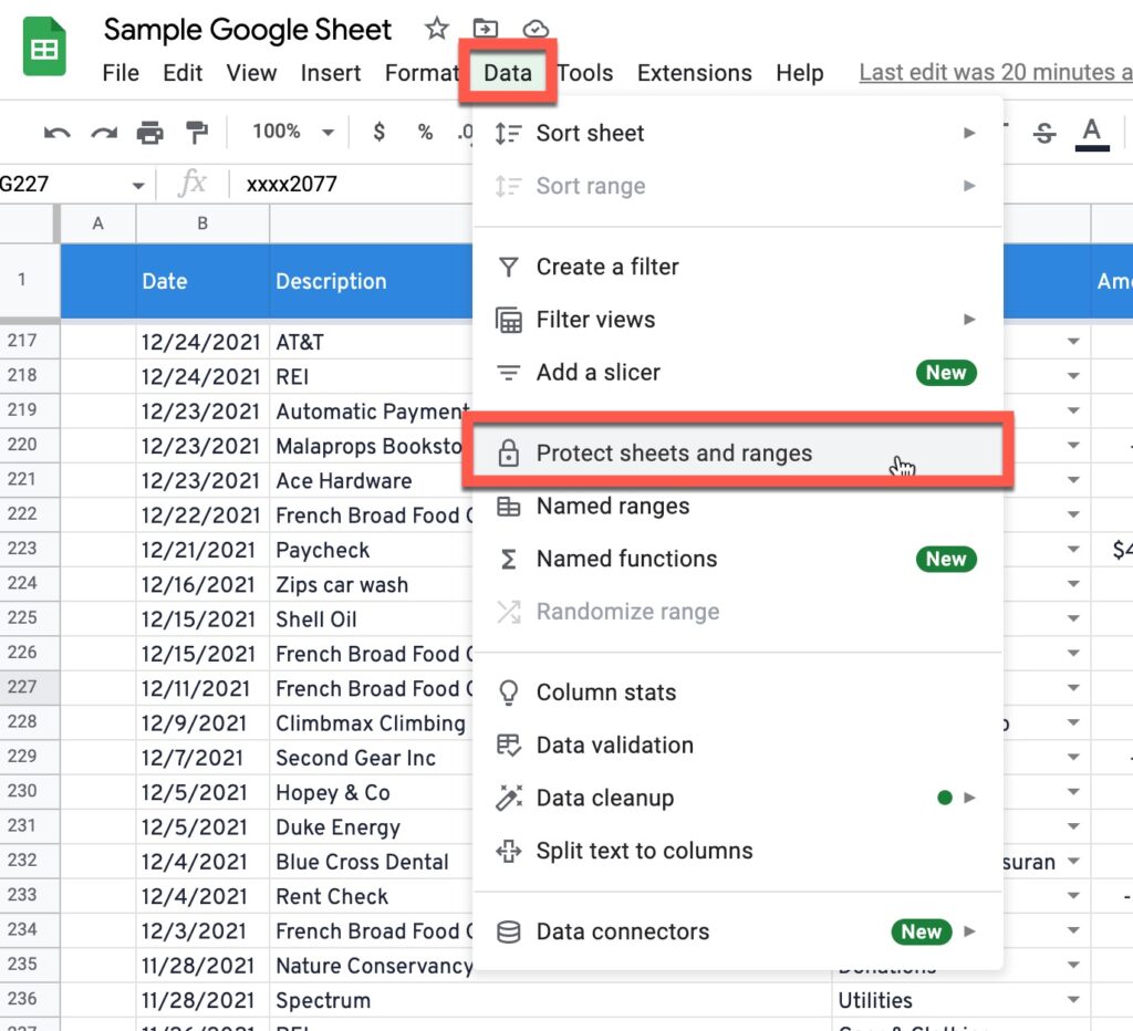
First, in the main menu, go to Data -> Protect sheets and ranges as shown in the screenshot above.

Click on the range entry you wish to change or delete

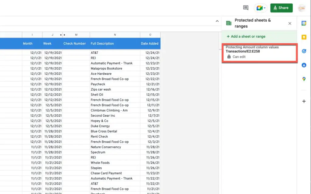
Click on the protected range you want to edit or remove permissions for

Next, you should see a list of the protected ranges and/or sheets on the right-hand panel as shown above. Click on the protected range you want to edit or remove.

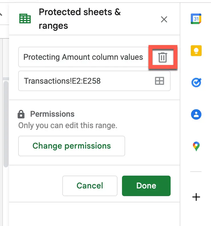
If you want to remove the protection from the range, click on the trash can button as shown above.

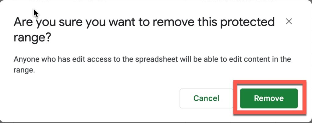
Click "Remove" button to delete cell range protection — Click the “Remove” button to delete cell range protection

A dialog box will appear asking you if you are sure you want to remove the protected range. If you are sure, click the “Remove” button as shown above.

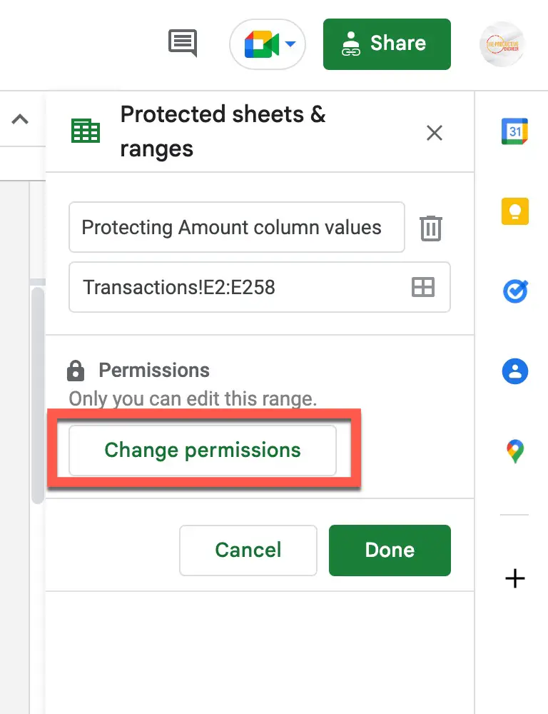
to edit the permissions of a protected range, click on the range and click the "Change permissions" button — to edit the permissions of a protected range, click on the range and click the “Change permissions” button

If you want to edit the existing permissions, simply click on the “Change permissions” button and change the permissions accordingly.

How Do I Use Google Apps Script to Lock Formatting in Google Sheets?

Google Apps Script is a feature of Google Docs that allows users to write code that can complete certain tasks as defined by the code that they have written. Google Apps Script is integrated will all Google Docs formats and so can be used to make changes to a sheet automatically.

There is a feature within Google Apps Script called ‘triggers.’ These allow a script to be executed at regular intervals or when a certain action is performed.

You can use this functionality to create a workaround to the problem of Google Sheets not supporting locking formatting only. In order to do this, you can take the following approach:

Attach a Google Apps Script to our Google Sheet
Create a protected range with the same formatting you wish to preserve across other cells
Create an onEdit function, which will execute whenever a cell is edited
Have the function:
- Copy the formatting from the protected range
- Paste the formatting to the editable range

This will ensure that even if users edit the formatting of the range as well as the value, the script will automatically reapply your desired formats — effectively locking the formatting of the selected cells.

How Do I Paste Values Without Changing Formatting in Google Sheets?

By far, the most common way that the formatting of a cell is changed accidentally is through the pasting of data from somewhere else. This is because the basic paste command pastes both the values and the formatting from your source.

It’s very easy to instruct Google Sheets to paste only the values from your clipboard onto the Google Sheet. This leaves the formatting of the target sheet untouched. There are two ways to achieve this.

Selecting from the menu
Using the keyboard shortcut

Selecting From The Menu

Once your desired data has been copied to your clipboard, select the cell range onto which you wish to paste your data. You can then click on Edit on the menu before selecting Paste special, and lastly, select Values only.

Using the Keyboard Shortcut

If you followed along with reviewing the menu, you might have seen that next to the Values only option is a snippet that shows a keyboard shortcut as a combined set of keystrokes. This is what you need to use to paste only the values from our keyboard without needing to go into the menu.

The keystroke you need will be slightly different depending on whether we’re on a PC or a Mac. On a PC, the keystroke is Control + Shift + V. On a Mac, the keystroke is Command + Shift + V.

Pressing these keys is equivalent to making the selection in the menu, and so again, once your data is ready on your clipboard, you just need to select your target range before pressing the keystroke, and the values should be pasted in.

Conclusion

Google Sheets is a powerful tool for fulfilling many business and personal applications. Being aware of both its features and limitations will enable you to create a perfectly formatted spreadsheet to meet your use case.