25 Awesome Tips for Microsoft Excel
Microsoft Excel is renown for its data management and spreadsheet functionality. It can handle a lot of crucial data with ease and precision. Microsoft Excel is extremely flexible and there are a lot of ways we can use it. Excel is unsurpassed in terms of feature-functionality. It follows that Excel is the go-to tool for anyone looking to analyze data.
This blog post will give you 25 cool tips for using Excel. These tips and tricks will help you in your day-to-day use of Excel. My hope is that a couple of these tips help you become more productive and efficient using Excel. Listed below are 25 Tips for Using Microsoft Excel:
1. Interchange Columns into Rows
2. Hiding a Cell
3. Freeze Row or Column Headings
4. Drag Cell to Copy Value to Other Cells
5. Deleting Blank Cells from a Column
6. Using Flash Fill in Excel
7. Adding Comments to Custom Formulas
8. Using the SUM Function
9. Rotate Heading Text
10. Add Decimal Points Quickly
11. Saving Charts as Template
12. Adding Calculator in Toolbar
13. Applying Conditions
14. Sketching Equations
15. Fast Navigation
16. Adding Values Starting from 0
17. Rename sheet quickly
18. Using & Symbol
19. Transform Text Case
20. Autocorrect Function
21. Generate Random Value
22. Input Restrictions
23. Applying Diagonal Borders
24. Adding More than one Row or Column
25. Some Important Shortcut Keys
Interchange Columns into Rows
In Excel, it’s possible to interchange data from Columns into Rows and vice versa. If you’ve accidentally put data in the wrong format, then you can easily interchange it.
It’s pretty simple. To interchange columns into rows in Excel, do the following:
- Copy the block of Cells you want to interchange.
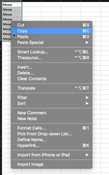
2. Right-click on the destination cell
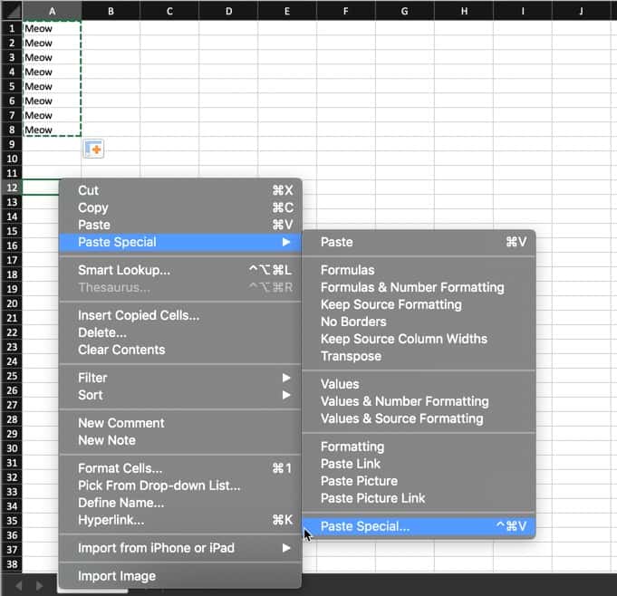
3. Choose Paste Special -> Paste Special
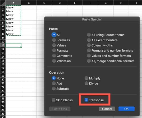
4. The Paste Special menu will appear, check the Transpose box and click Ok

Congratulations! You’ve interchanged cells successfully.
Hiding a Cell
There are a lot of tricks in Excel. One of them is hiding cells. It can be convenient to hide certain cells when working in a spreadsheet. Doing so is straightforward.
To hide a cell or cells in Excel, follow the steps listed below:
Select the cell(s) you want to hide
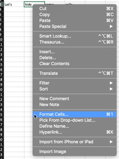
Right-click and select Format Cells
Click on the Number tab
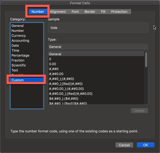
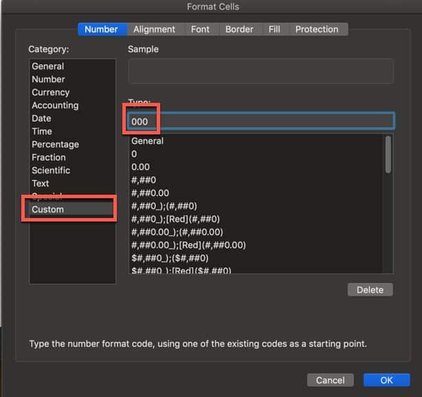
Set the format as Custom
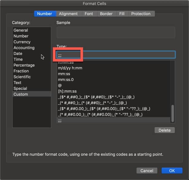
In the Type text bar, type “;;;” and click Ok
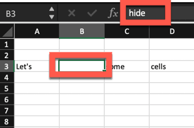
If you look at the screenshot above, the cell (B3) shows blank in the sheet but when you click on the cell, the value does appear in the cell entry text box. This works where it is text, numbers or even formulas.
Freeze Rows or Column Headings
This is a simple yet very useful trick to use in Excel. You can freeze the row and column headings. Therefore, no matter how much you scroll you will still see these rows and columns. This trick is rather simple to implement.
To freeze a row or column heading in Excel, do the following:
- Open your spreadsheet
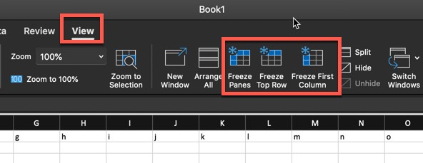
2. Click on the View Tab and select one of the following options:
- Freeze Panes – Freezes the top row and first column
- Freeze Top Row – Freezes the top row
- Freeze First Column – Freezes first column
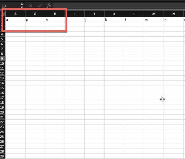
Your first row and/or column will be visible as you scroll.
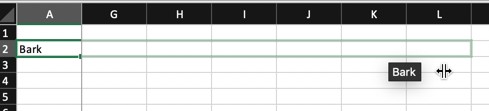
Drag Cell to Copy Value to Other Cells
If you need to copy the value of a cell to neighboring cells, here is a quick tip. Excel allows you to quickly copy the value of a cell to neighboring cells by dragging the corner of the cell.
To copy the value of a cell to neighboring cells in Excel, do the following:
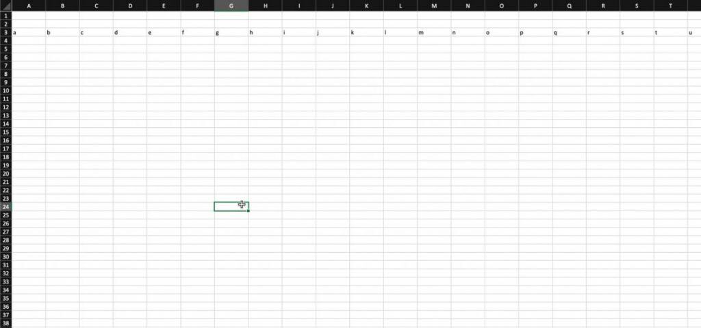
- Select the Cell you want to copy.
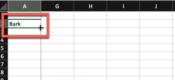
- Hover over the corner of the cell until the cursor turns into a crosshair.
- Click and drag the cell across the cells you want to copy to.
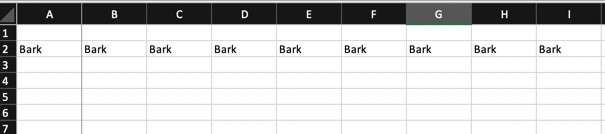
- Release the mouse button and the value of the original cell will be copied into all of the destination cells.
Deleting Blank Cells from a Column
When working with a column of data, there can be blank values in some of the cells. Sometimes, you might want to delete all the cells with blank values in a given column. This functionality is easily achievable in Excel.
To delete blanks cells in a column in Excel, do the following:
Select the column that you want to use
Click on the Data tab
Click on the Filter button. This will add a filter drop-down to the top cell of your column.
Uncheck Select All
Scroll to the bottom of the list and check (Blanks)
The cells with blank values should be the only lines showing and the row numbers should be in a different color.
Select the colored row numbers by holding down the Shift key and selecting the first and last row. Go to Home and click on the Delete button. This will remove the rows.
Undo your filter by clicking on the drop-down button in the top cell of your column and check Select All.
Your column should have all of your values minus the blank cells.
Using Flash Fill in Excel
Excel is a really intelligent application. One of the ways Excel is intelligent is that it can sense patterns in data entry. This is really useful when you want to fill a bunch of cells that follow a specific pattern.
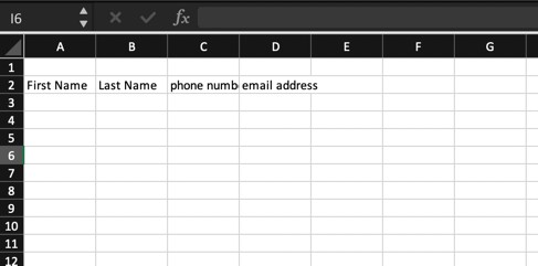
An example of this functionality would be in a contact spreadsheet where you have the full name and email handle and need to populate separate columns for first and last name. We will use this example to show how Flash Fill works. To use the Flash Fill feature in Excel, do the following:
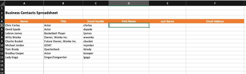
Open the spreadsheet you want to use

Fill in the first row of your spreadsheet with the information you want to flash fill for the other cells
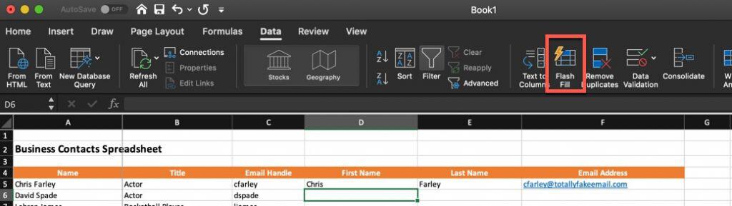
Click on the next cell below the filled-in cell and go to Data. Press the Flash Fill button.
This feature can be a great time saver as it minimizes repetitive data entry.
Adding Comments to Custom Formulas
Excel allows you to create custom formulas to calculate values. Depending on the sophistication of the formula, it may make sense to add some comments to clarify what the formula is doing. Excel supports the ability to add comments to formulas using the N() function.
To add comments to a formula in Excel, do the following:
Write your formula
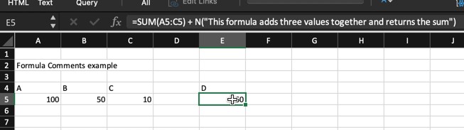
At the end of your formula, append the formula by typing + N(“Comments”) where Comments are your actual comments.
The value of the cell will remain the result of your formula but now you have an in-formula comment explaining the logic of your formula.
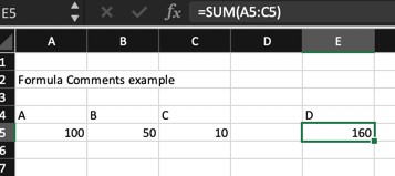
Using the SUM Function
Adding a list of value up is a core feature of any spreadsheet. I find myself constantly summing a column or row of values. Excel has a wide variety of built-in functions but the most commonly used one, for me, is the SUM function. The SUM function calculates the sum of a list of values.
To use the SUM function in Excel, do the following:
Click on the cell where you want the sum to display
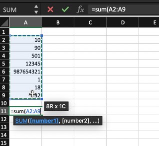
Type =sum( and then select the cells you want to add together and press Enter
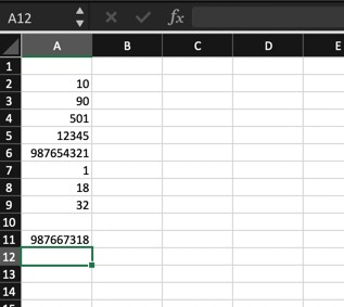
The sum of the selected numbers should now appear in your cell.
Rotate Heading Text
While we are all used to entering our column headings as horizontal entries, it can be valuable to have your column heading be vertical. Excel makes it easy to rotate your column headings. To rotate your column headings, do the following:
Select the cells you want to rotate
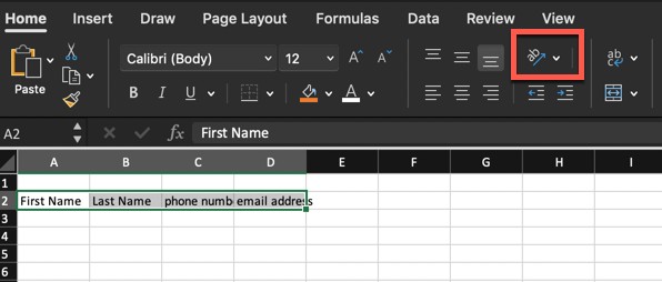
Go to the Home tab and click on the Orientation button
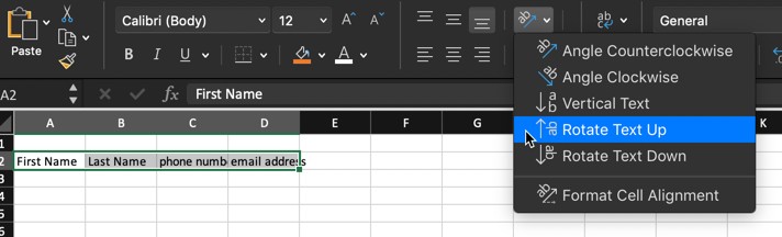
From the sub-menu, select the Orientation you want
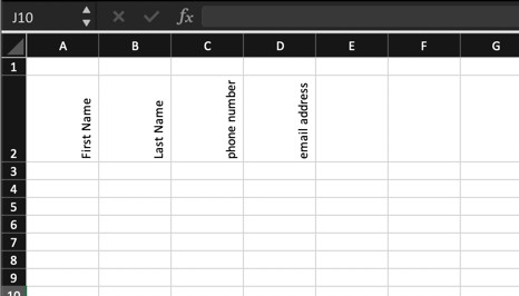
Your cells should now have the desired orientation.
Add Decimal Points Quickly
Working in Excel, you typically will need to use decimal numbers, whether it’s currency or simply calculating values with decimal precision. Excel excels (forgive the pun) at formatting values. To format the value to a set level of decimal precision, do the following:
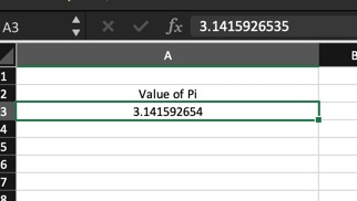
Select the cell you want to set the decimal precision for.
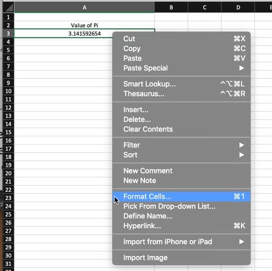
Right-click on the cell and select Format Cells…
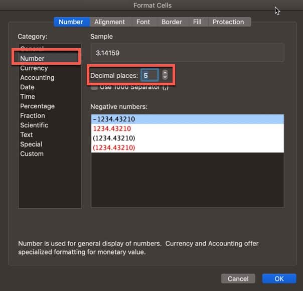
Click on Number in the Category section and at the Decimal places text box, type in the number of decimal places the cell should display. Press Ok when done.

Your cell should display the number with the number of decimal places you set.
Saving Charts as Templates
This trick can make you feel like a master of Excel. You can save a combination of layout and colors which you think are pretty important to you,
The significance of saving as a template is that you can use the template again and again if you want. To save a chart as a template in Excel, do the following:
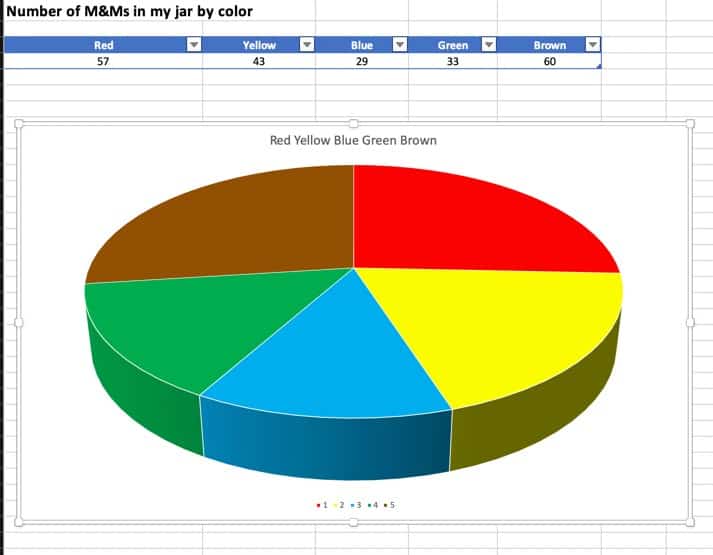
Select the chart you want to save as a template
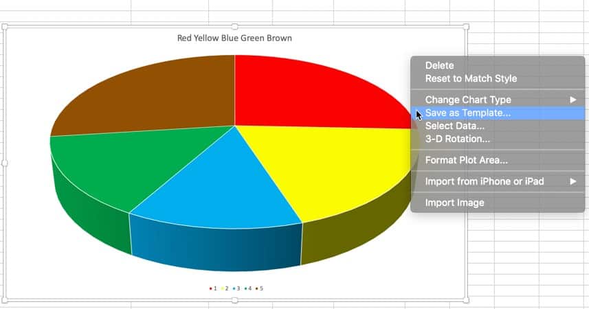
Right-click on the chart and select Save as Template…
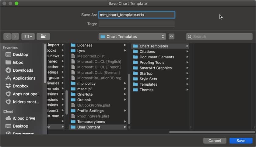
Type in the name you want to assign to your template and press Save.
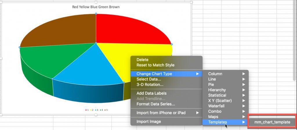
Your chart template is now available as a formatting option for your future charts. This is helpful if there is a color scheme you like as an example.
Add Calculator in Toolbar
Excel gives you several shortcut controls. For example, you can add shortcuts such as calculators, camera or other apps. Shortcuts provide simplified access to the tools you most commonly use.
To create a custom shortcut in Excel, do the following:

Click on the drop-down arrow at the top of your Excel window
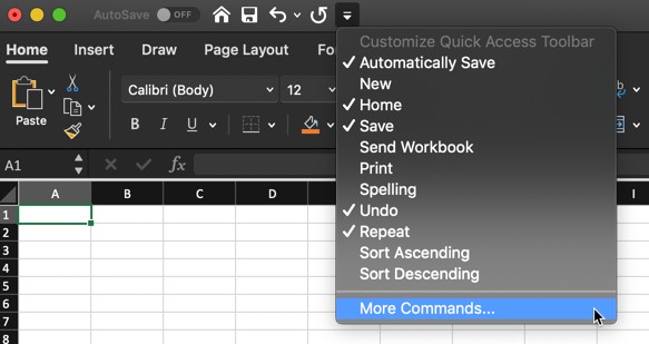
Scroll down to the bottom of the menu and select More Commands…

Select the command(s) you want to add to your toolbar and press the > arrow button and press Save.
Your command will now be available for use in the Quick Access Toolbar.
Apply Conditions
Excel provides you the options to set certain conditions and rules for your cells. You can do this by adding conditional formatting. It’s really simple to use.
To set up conditional formatting in Excel, do the following:
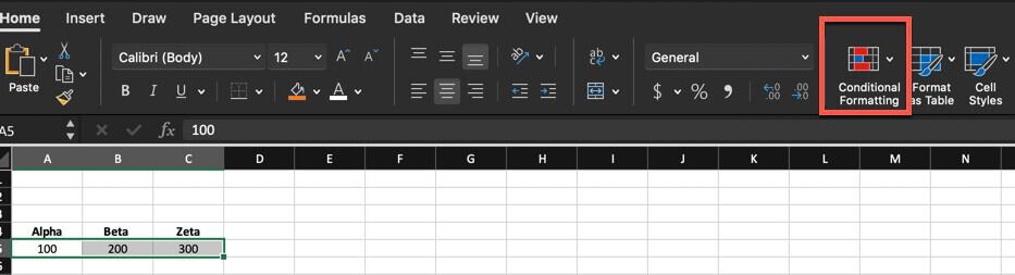
Select the cells you want to format and press the Conditional Formatting button.
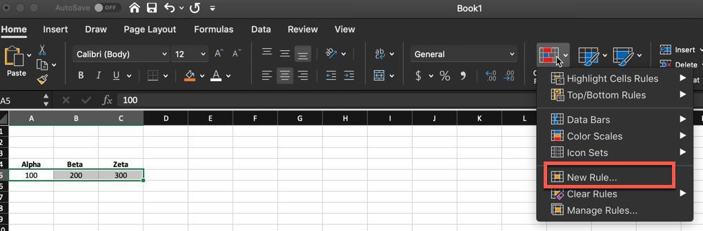
There are a bunch of formatting options you can choose from. For this demo, we will choose New Rule…
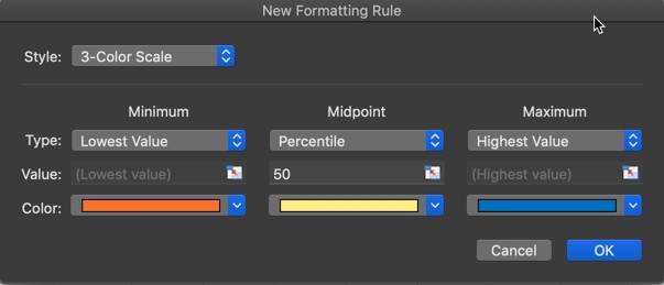
Pick your style and criteria using the Style and Type controls and press OK when done.

Your cells should have the formatting you specified.
Sketching Equations
This feature of Excel 2016 or later (Windows only) allows you to draw equations. This is very useful if you have a touchscreen laptop or pc. It’s pretty simple to do.
To draw equations in Excel for Windows, do the following:
- Click on the Insert Tab
- Select Equation
- Select Ink Equation
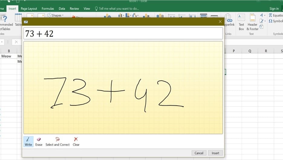
After that, a yellow box will appear. You can start drawing in the yellow box. The yellow box automatically detects what you’ve typed in that box.
Fast Navigation
It’s often tiring trying to go down to the last cell. Rather than having to scroll through a bunch of rows, Excel has made it easy for you.
To quickly navigate to the last populated cell in an Excel worksheet, do the following:
Open the worksheet

Press the keyboard shortcut for your platform from the table below
| Platform | Keyboard Shortcut |
| Window | CTRL + Down Arrow |
| Mac | Command + Down Arrow |

Adding Values Starting with 0
Let’s say that you want to input numbers that start with zero. An example where you might want to do this is for creating invoice numbers. The problem is, by default, Excel automatically deletes the lead zero(es) from numbers that start with zero.
However, you can configure the cells to support lead zeroes.
To enable lead zeroes for numbers in Excel, do the following:
Select the cell(s) you want to enable lead zeroes for
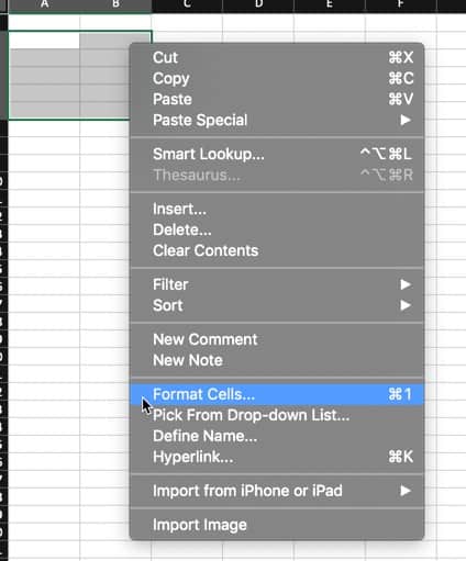
Right Click on the cells and select Format Cells
Select Custom and in the Type text box, enter the number of zeros to accommodate the max value you want to support. For example, if you want the ability to support a max of 999 values, you would enter three zeroes. Once you have entered the numbers, click Ok.
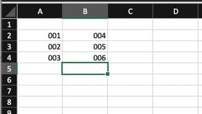
If you type in a number, it will add the zeroes automatically as shown above.
Rename Sheet Quickly
Renaming a worksheet in Excel is really easy. Simply do the following:
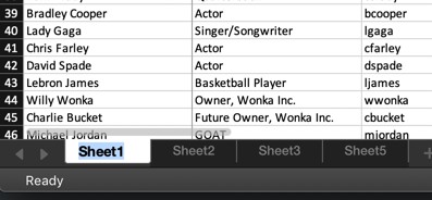
Double-click on the worksheet tab
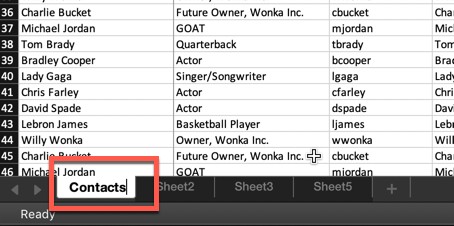
Type in the name you want to assign the worksheet and press Enter.
Using the & Symbol
The & sign is a pretty useful operator in programming languages. But in Excel, it’s used to concatenate (join) strings together. Consider you got 3 cells. Each has a different string. You want to make one string out of them. Excel supports this using the & symbol.
To concatenate text strings in Excel, do the following:
In the worksheet that you want to use, click on an open cell
Type = and select the first cell. Add the & symbol. This tells Excel that there will be another string being added. If you want a space between the strings you are combining, use ” ” to add a space.
An example of combining three strings with a space between each string would look like the equation below:
=A5&” “&B5&” “&C5
A5, B5, and C5 are the cell references for each string.

Transform Text Case
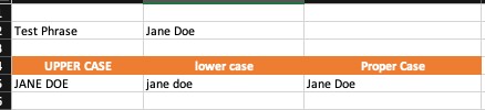
Excel allows you to convert the case of the text in a cell to the following:
- Uppercase -> all characters are UPPERCASE
- Lowercase -> all characters are lowercase
- Proper case -> Only the first character of each word is capitalized
Excel accomplishes this using the UPPER, LOWER and PROPER functions.
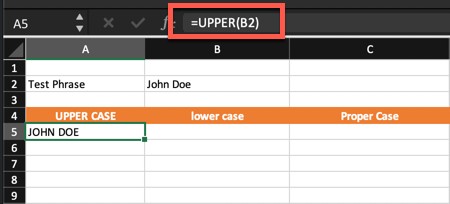
To set the text to uppercase in Excel, use the UPPER function.

To set the text to lowercase in Excel, use the LOWER function.
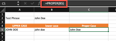
To set the text to proper case in Excel, use the PROPER function.
Autocorrect Function
Sometimes you might want to replace one string of text with another throughout your spreadsheet. Excel supports autocorrection.
To setup autocorrect in Excel for Mac, do the following:
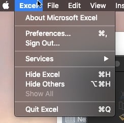
Go to Excel -> Preferences in Main Menu
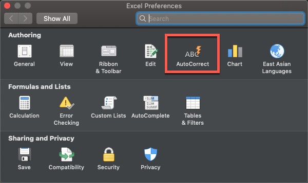
Select AutoCorrect
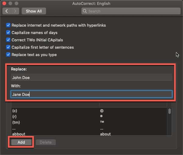
Type in the character or string you want to replace in the Replace text box and the replacement string in the With text box and press Add.
Now, when you type the original phrase, it will be automatically replaced with the new phrase. In my example, everytime I type “John Doe”, Excel replaces it with “Jane Doe”.
Generate Random Values
You can generate unique values in Excel. To create a random number in Excel, do the following:
Click on the cell you want to use to create the random number
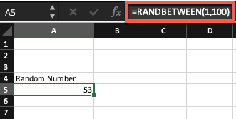
Type in =RANDBETWEEN(x,y) where the random number will be between x and y. For example, if you wanted a random number between 1 and 100, you would type:
=RANDBETWEEN(1,100)
Input Restrictions
In some cases, you want to validate inputted data to ensure it complies with the expected data type of the cell. Consider an example of a date of birth. It shouldn’t contain any characters. Excel provides the ability to define your own conditions.
To create input restrictions in Excel, do the following:
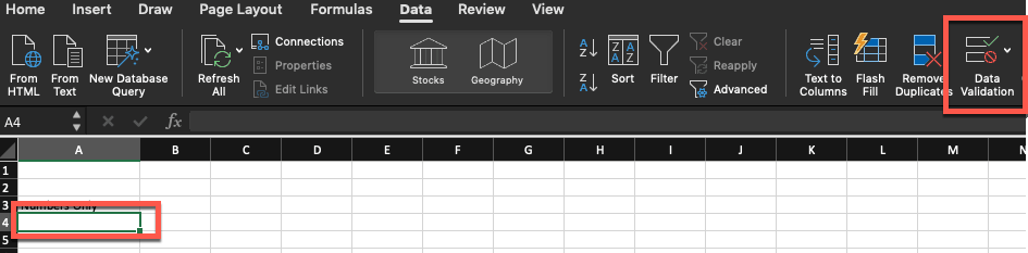
Click on the Data tab and select Data Validation
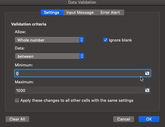
In the Allow drop-down menu, choose your allowed input type. If choosing a number, define the range of values you will allow. Then click the Input Message tab.
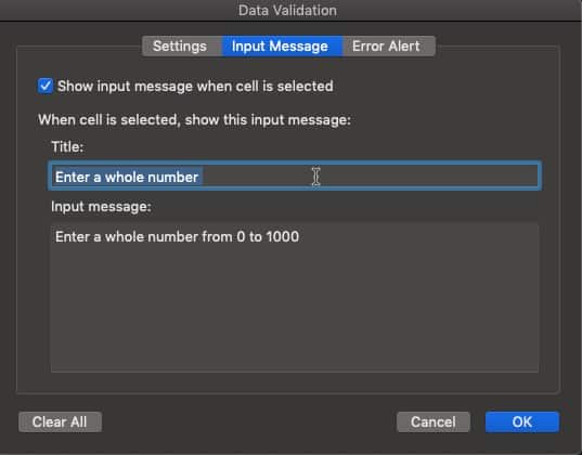
Excel allows you to define an input message that will inform your users of what values are acceptable. Enter the input message and title and click on the Error Alert tab.
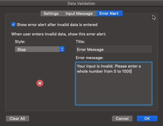
The Error Alert tab allows you to configure an error message that will be displayed to the user if they attempt to enter an invalid value. Type in your error message and it’s title and press Ok.
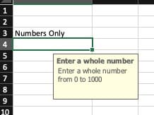
When you click on the cell, your input message will display.
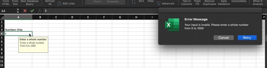
If you attempt to type in an invalid value, your custom error will pop-up and instruct the user appropriately.
Applying Diagonal Borders
Most people know that you can add borders to cells in Excel. However, you can also add diagonal borders as well. To add diagonal borders in Excel, do the following:
Select the cells you want to apply diagonal borders to
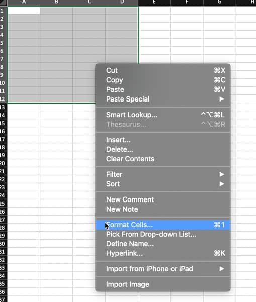
Right-click on the cells and select Format Cells…
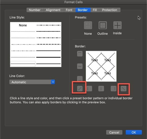
Go to the Border tab and click on the diagonal border buttons. Press Ok.
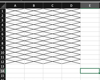
Your cells will now have diagonal borders.
Adding More than One Row or Column
A lot of users add rows or columns one row or column at a time. But if you want to add multiple rows or columns, there is an easy way to do it. To add more than one column or row at one time, do the following:
Click on the row or column where you want to add and drag until you have the number of row/columns you want to add
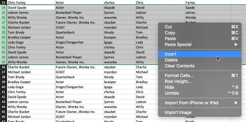
Right-click and select Insert from the drop-down menu
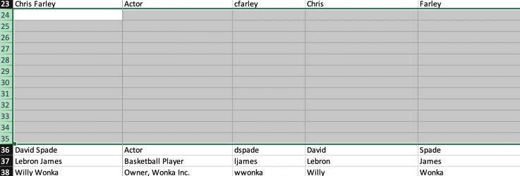
These new rows will be inserted into the desired position.
Some Important Keyboard Shortcuts
There are some essential keyboard shortcuts you really should know in Excel. I have created the table below that contains some of my favorites:
| Function | Windows Keyboard Shortcut | Mac Keyboard Shortcut |
| Jump from first to last or last to first | CTRL-UP/DOWN | COMMAND-UP/DOWN |
| Save your spreadsheet | CTRL-S | COMMAND-S |
| Create a chart | ALT-F1 | OPTION-F1 |
| Create a new workbook | CTRL-N | COMMAND-N |
| Open A New Workbook | CTRL-O | COMMAND-O |
| Open Format Cells menu | CTRL-1 | COMMAND-1 |
| Add or remove a filter | CTRL-SHIFT-L | COMMAND-SHIFT-L |
| Hide selected rows | CTRL-9 | CONTROL-9 |
Want More Tips and Tricks? Subscribe to our Newsletter!
If you haven’t already subscribed, please subscribe to The Productive Engineer newsletter. It is filled with tips and tricks on how to get the most out of the productivity apps you use every day. We hate spam as much as you do and promise only to send you stuff we think will help you get things done.
Check Out Our YouTube Channel!
We have a YouTube channel now and we are working hard to fill it with tips, tricks, how-tos, and tutorials. Click the link below to check it out!
Resources Page
Check out our resources page for the products and services we use every day to get things done or make our lives a little easier at the link below:
Article You May Be Interested In
Ten Great Tips for Using Todoist
Link to Ten Great Tips for Using Todoist
A Beginner’s Guide to Trello
Link to A Beginner’s Guide to Trello
7 Ways to Overcome Impostor Syndrome
Link to 7 Ways to Overcome Impostor Syndrome